free flow travel speeds

Tradeoffs among free-flow speed, capacity, cost, and environmental footprint in highway design

• Published: 12 April 2012
• Volume 39 , pages 1259–1280, ( 2012 )

Cite this article

• Chen Feng Ng 1 &
• Kenneth A. Small 2  

903 Accesses

14 Citations

6 Altmetric

Explore all metrics

This paper investigates differentiated design standards as a source of capacity additions that are more affordable and have smaller aesthetic and environmental impacts than modern expressways. We consider several tradeoffs, including narrow versus wide lanes and shoulders on an expressway of a given total width, and high-speed expressway versus lower-speed arterial. We quantify the situations in which off-peak traffic is sufficiently great to make it worthwhile to spend more on construction, or to give up some capacity, in order to provide very high off-peak speeds even if peak speeds are limited by congestion. We also consider the implications of differing accident rates. The results support expanding the range of highway designs that are considered when adding capacity to ameliorate urban road congestion.

This is a preview of subscription content, log in via an institution to check access.

Access this article

Subscribe and save.

• Get 10 units per month
• Download Article/Chapter or eBook
• 1 Unit = 1 Article or 1 Chapter
• Cancel anytime

Price includes VAT (Russian Federation)

Instant access to the full article PDF.

Rent this article via DeepDyve

Institutional subscriptions

Similar content being viewed by others

Redesigning an Urban Midblock Section to Improve Safety and Level of Service: Case Study in the Niagara Region

Urban Road Design and Keeping Down Speed

See FHWA ( 2006 ), Ch 7. Of the $84.5 billion in investments in urban arterial and collector roads meeting defined cost-benefit criteria in this report, 53% is for freeways and expressways—of which about half is for expansion, half for rehabilitation or environmental enhancement (Exhibit 7-3).

We do not attempt to account quantitatively for the truck restrictions, tighter curves, or nicer landscaping that may further enhance parkway amenities. We suspect that in some cases it would be optimal to restrict trucks altogether, but an explicit model of truck restrictions would be far more complex and is not undertaken here. Safety implications are discussed further in the section on “Safety”.

Cassidy and Bertini ( 1999 ) suggest that the highest observed flow, which is larger, is not a suitable definition of capacity because it generally breaks down within a few minutes—although Cassidy and Rudjanakanoknad ( 2005 ) hold out some hope that this might eventually be overcome through sophisticated ramp metering strategies. Our speed-flow function does not include the backward-bending region, known as congested flow in the engineering literature and as hypercongested flow in the economics literature, because flow in that region leads to queuing which we incorporate separately. See Small and Verhoef ( 2007 , Sect 3.3.1, 3.4.1) for further discussion of hypercongestion.

Analyzing more daily time periods would of course increase precision, but would also make the model more location-specific. By using only two periods, we miss some congestion that is caused by queue buildups during shorter periods of higher demand, and thus may understate the advantage of higher-capacity roads. To compensate, we use a rather long 4-h one-directional peak.

We ignore the difference in cost due to converting part of the paved shoulders in the “regular” design to vehicle-carrying pavements in the “narrow” design; since the largest component of new construction cost is grading and structures, this difference should be minor. We also ignore any differences in maintenance cost that may occur because vehicles on narrow lanes are more likely to veer onto the shoulder or put weight on the edge of the pavement (AASHTO 2004 , p. 311).

Note that for the urban streets in Fig.  3 b, the total two-directional roadway width at the intersection itself is less than the sum of those of the two separate one-directional roadways, because the left turn lanes in both directions share the same lateral space. That is, the width of the two directional roadway includes only the width of one, not two, left turn lanes. For the “regular” design this is 2 × (12 + 12 + 8) + 12 = 76 = 2 × 38, whereas for the “narrow” design it is 2 × (10 + 10 + 10 + 3) + 10 = 76 = 2 × 38; hence both are described as having a 38-foot one-directional roadway.

The calculations are done with each period continuous (i.e. 6–10 am peak, 10 am–10 pm offpeak). We found it makes a negligible difference if the peak is in the afternoon so the offpeak period is split into two parts. We also computed results for a two-peak scenario with each peak period equal to 2 h, representing a case where the traffic is evenly distributed during the morning and afternoon peaks. The two-peak scenario is briefly addressed at the end of this and the next sections, and both results are described in detail in Appendix B of the Online Resource.

Nevertheless, we performed the same analysis using reconstruction costs of existing lanes, which are lower than the construction costs of new alignment shown in Table  3 . The results are qualitatively similar: using reconstruction costs favors the narrow roads somewhat less in small cities and more in large cities. The sources used are the same as those listed in Table  3 ; see Appendix C of the Online Resource for more details.

Lake Shore Drive includes six signalized intersections (only five going southbound) within its 15-mile length, for an average spacing of over two miles; but all the signals are within a central section about 2.4 miles in length. This highway opened in 1937 (Chicago Area Transportation Study 1998 ).

Of course, the idea of building an entire network is an idealization, made here solely in order to account for the different capacities of different design options.

According to Small and Verhoef ( 2007 , Sect. 2.6.5), the value of time for work trips is typically estimated as 50% of the wage rate, which would be about $10.50 per hour for 2009 (BLS 2010 , Table 1, reporting mean hourly wage for civilian workers). We assume these value of time studies apply to the entire vehicle, although authors are often ambiguous. Values of time are higher for work trips than for others, but occupancies are lower; we assume these two factors balance out between peak and off-peak travel so assign them both the same value of time.

The delay calculation in the bottleneck queuing model at the entrance of the road is very similar to the HCM’s control delay. In the bottleneck model described in Section 2 of this paper, the uniform control delay is zero (because there is no signal) and the term containing k in Eq. ( 16 ) is negligible because of the large traffic volume. The remaining components in Eq. ( 16 ) plus the HCM initial queue delay (both converted to hours) give precisely the same result as the bottleneck model.

AASHTO: A Policy on Geometric Design of Highways and Streets, 5th edn. American Association of State Highway and Transportation Officials, Washington (2004)

Google Scholar  

AASHTO: A Policy on Design Standards: Interstate System, 5th edn. American Association of State Highway and Transportation Officials, Washington (2005)

Alam, M., Kall, D.: Improvement Cost Data: Final Draft Report. Prepared for the Office of Policy, Federal Highway Administration (2005)

Alam, M., Ye, Q.: Highway Economic Requirements System Improvement Cost and Pavement Life: Final Report. Prepared for the Office of Policy, Federal Highway Administration (2003)

Bauer, K.M., Harwood, D.W., Hughes, W.E., Richard, K.R.: Safety effects of narrow lanes and shoulder-use lanes to increase capacity of urban freeways. Transp. Res. Rec. 1897 , 71–80 (2004)

Article   Google Scholar  

BLS (2010) National compensation survey: occupational earnings in the United States, 2009. Bureau of Labor Statistics, Washington. http://www.bls.gov/ncs/ncswage2009.htm . Accessed May 2011

Cassidy, M.J., Bertini, R.L.: Some traffic features at freeway bottlenecks. Transp. Res. B-Meth. 33 , 25–42 (1999)

Cassidy, M.J., Rudjanakanoknad, J.: Increasing the capacity of an isolated merge by metering its on-ramp. Transp. Res. B-Meth. 39 , 896–913 (2005)

Chicago Area Transportation Study: 1995 Travel Atlas for the Northeastern Illinois Expressway System. Chicago Area Transportation Study, Chicago (1998)

Downs, A.: The law of peak-hour expressway congestion. Traffic Quar. 6 , 393–409 (1962)

Downs, A.: Still Stuck in Traffic: Coping with Peak-Hour Traffic Congestion. Brookings Institution Press, Washington (2004)

FHWA: Highway performance monitoring system field manual. Federal Highway Administration, Washington (2002). http://www.fhwa.dot.gov/ohim/hpmsmanl/hpms.htm . Accessed August 2008

FHWA: Price trends for federal-aid highway construction. Federal Highway Administration, Washington (2003). http://www.fhwa.dot.gov/programadmin/pt2003q1.pdf . Accessed May 2011

FHWA: Status of the nation’s highways, bridges, and transit: conditions and performance. Federal Highway Administration, Washington (2006). http://www.fhwa.dot.gov/policy/2006cpr/ . Accessed August 2008

FHWA: National highway construction cost index. Federal Highway Administration, Washington (2011). http://www.fhwa.dot.gov/policyinformation/nhcci.cfm . Accessed May 2011

Fridstrøm, L.: An Econometric model of car ownership, road use, accidents, and their severity. TØI Report 457/1999. Institute of Transport Economics, Oslo (1999). http://www.toi.no/getfile.php/Publikasjoner/T%D8I%20rapporter/1999/457-1999/457-1999.pdf . Accessed August 2008

Harwood, D.W., Bauer, K.M., Richard, K.R., Gilmore, D.K., Graham, J.L., Potts, I.B., Torbic, D.J., Hauer, E.: Methodology to predict the safety performance of urban and suburban arterials. National cooperative highway research program web-only document 129: Phases I and II. (2007) http://onlinepubs.trb.org/onlinepubs/nchrp/nchrp_w129p1&2.pdf . Accessed January 2012

Hu, P.S., Reuscher, T.R.: Summary of Travel Trends: 2001 National Household Travel Survey. Federal Highway Administration, Washington (2004). http://nhts.ornl.gov/2001/pub/STT.pdf . Accessed May 2011

Ivan, J.N., Garrick, N.W., Hanson, G.: Designing roads that guide drivers to choose safer speeds. Report No. JHR 09-321. Connecticut Department of Transportation, Rocky Hill, Connecticut (2009)

Kweon, Y., Kockelman, K.M.: Safety effects of speed limit changes: use of panel models, including speed, use, and design variables. Transp. Res. Rec. 1908 , 148–158 (2005)

Lewis-Evans, B., Charlton, S.G.: Explicit and implicit processes in behavioural adaptation to road width. Accid. Anal. Prev. 38 , 610–617 (2006)

Liu, R., Tate, J.: Network effects of intelligent speed adaptation systems. Transportation 31 , 297–325 (2004)

Lord, D., Middleton, D., Whitacre, J.: Does separating trucks from other traffic improve overall safety? Transp. Res. Rec. 1922 , 156–166 (2005)

Mirshahi, M., Obenberger, J., Fuhs, C.A., Howard, C.E., Krammes, R.A., Kuhn, B.T., Mayhew, R.M., Moore, M.A., Sahebjam, K., Stone, C.J., Yung, J.L.: Active traffic management: the next step in congestion management. Report No. FHWA-PL-07-012. American Trade Initiatives, Alexandria, Virginia (2007) http://international.fhwa.dot.gov/pubs/pl07012/ . Accessed August 2008

Office of Management and Budget: Guidelines and discount rates for benefit-cost analysis of federal programs. Circular no. A-94, revised, Section 8. US Office of Management and Budget, Washington (1992)

Peltzman, S.: The effects of automobile safety regulation. J. Polit. Econ. 83 , 677–725 (1975)

Pigou, A.C.: The Economics of Welfare. Macmillan, London (1920)

Small, K.A., Verhoef, E.T.: The Economics of Urban Transportation. Routledge, London (2007)

Transportation Research Board: Highway Capacity Manual 2000. Transportation Research Board, Washington (2000)

Zegeer, J.D., Vandehey, M., Blogg, M., Nguyen, K., Ereti, M.: Default values for highway capacity and level of service analyses. National Cooperative Highway Research Program Report 599. Transportation Research Board, Washington (2008)

Download references

Acknowledgments

We are grateful to the University of California Transportation Center for financial support, and to three anonymous referees and many colleagues for comments on earlier drafts, especially Pablo Durango-Cohen, Robin Lindsey, Robert Noland, Robert Poole, Peter Samuel, Ian Savage, and Erik Verhoef. Of course, all responsibility for facts and opinions expressed in the paper lies with the authors.

Author information

Authors and affiliations.

Department of Economics, California State University Long Beach, 1250 Bellflower Blvd, Long Beach, CA, 90840-4607, USA

Chen Feng Ng

Department of Economics, 3151 Social Science Plaza, University of California at Irvine, Irvine, CA, 92697, USA

Kenneth A. Small

You can also search for this author in PubMed   Google Scholar

Corresponding author

Correspondence to Chen Feng Ng .

Electronic supplementary material

Below is the link to the electronic supplementary material.

Supplementary material 1 (PDF 458 kb)

Appendix: speeds and capacities from the highway capacity manual (2000).

This appendix briefly discusses the HCM’s methodology for calculating speeds and capacities for expressways, which the HCM calls “freeways” (based on HCM ch. 13, 23), and arterials (based on HCM, ch. 10, 12, 15, 16, 21). A more detailed explanation of the equations and parameter values are presented in the online version of this Appendix (see Online Resource).

Expressways/Freeways

Capacity varies by free-flow speed, and equation 23-1 in the HCM is used to estimate free-flow speed (FFS) of a basic freeway segment:

A brief description of each parameter and the parameter values used in the paper are given in Table  5 . As shown in Appendix N of the highway performance monitoring system (HPMS) field manual (FHWA 2002 ), the relationship between base capacity ( BaseCap , measured in passenger-car equivalents per hour per lane) and free-flow speed is:

Equation 23-2 in the HCM is used to convert hourly volume V , which is typically in vehicles per hour, to v p , which is in passenger-car equivalents per hour per lane (pce/h/ln) and is used later on to estimate speed:

See Table  5 for the parameter values used in this paper. Equation ( 3 ) can also be used to calculate capacity in terms of vehicles per hour for all lanes, which we call V K in this paper, by replacing V   =   V K and v p  =  BaseCap.

We use the HCM speed-flow diagrams in Exhibit 23-3 to calculate average passenger-car speed S (min/h) as a function of the flow rate v p (pce/h/ln).

Urban arterials

The high-type unsignalized arterial analyzed in the comparison between freeways and arterials in Sect.  4 is an example of a “multilane highway” in the HCM’s terminology. The capacity and free-flow speed of this arterial are calculated using the procedures outlined in Chapters 12 and 21 of the HCM (which are very similar to the expressway calculations). However, we make the following modification to the HCM speed-flow function since the HCM function results in the high-type arterial having a higher speed at capacity than the expressway. For free-flow speeds between 55 and 60 min/h, that speed-flow function (Exhibit 21-3 of the HCM) is:

The high-type arterial’s speed at capacity (which we shall denote as \( S_{a}^{\text{cap}} \) ) can be calculated from this equation by setting flow rate v p equal to capacity. Denoting the expressway’s speed at capacity as \( S_{e}^{cap} \) , we then define a modified speed-flow function for the high-type arterial so that \( S_{a}^{\text{cap}} = S_{e}^{\text{cap}} \) , essentially by increasing the rate at which speed falls with traffic volume. Specifically we use:

where S a is given by equation ( 14 ).

For the signalized urban arterials in Sect.  3 (which the HCM calls “urban streets”; see Chapters 10, 15 and 16), we focus on high-speed principal arterials (design category 1). These arterials have speed limits of 45–55 min/h and a default free-flow speed of 50 min/h (Exhibits 10-4 and 10-5 of the HCM). Using the procedure recommended by Zegeer et al. ( 2008 , pp. 66–73), if we assume the speed limits on the “regular” and “narrow” arterials in Sect.  3 are 55 and 45 min/h respectively, this gives us free-flow speeds of 51.5 and 46.8 min/h.

A vehicle’s travel time on an urban street (ignoring queuing due to volumes exceeding capacity, computed separately in the text) consists of running time plus “control delay” at a signalized intersection. Based on Exhibit 15-3 of the HCM, running time for an urban arterial longer than one mile is calculated as the length divided by the free-flow speed.

The formula for calculating control delay (Eq. 16 – 9 in the HCM) is the sum of three components: (1) uniform control delay, which assumes uniform arrivals; (2) incremental delay, which takes into account random arrivals and oversaturated conditions (volume exceeding capacity); and (3) initial queue delay, which considers the additional time required to clear an existing initial queue left over from the previous green period. Footnote 12 Because the initial queue limits entry flow to the road’s capacity, the initial queue occurs only once at the entry to the road (prior to the first signal) since the traffic volume arriving at each intersection is never greater than the intersection’s capacity. As a result, the control delay in this paper consists only of uniform control delay and incremental delay. Using Eqs.  16 – 9 , 16 – 11 and 16 – 12 of the HCM, the control delay at a signal is:

Table  6 provides a description of the parameters and the values used in this paper.

The arterial’s capacity, V K , is based on the saturation flow rates of the through and shared right-turn/through lane groups, along with the fraction of time the signal is green and the proportion of traffic at each intersection that is making left turns. Saturation flow means the highest flow rate that can pass through the intersection while the light is green and is calculated based on equations  16 – 4 and 16 – 6 of the HCM. Saturation flow rates depend on the number of lanes, lane width, proportion of vehicles turning right, and other factors. For the most part, we use the default values recommended by the HCM and we assume that 7.5 % of the total traffic volume will be vehicles turning left, and similarly for vehicles turning right. Complete details are available in the online version of this Appendix (see Online Resource).

Rights and permissions

Reprints and permissions

About this article

Ng, C.F., Small, K.A. Tradeoffs among free-flow speed, capacity, cost, and environmental footprint in highway design. Transportation 39 , 1259–1280 (2012). https://doi.org/10.1007/s11116-012-9395-8

Download citation

Published : 12 April 2012

Issue Date : November 2012

DOI : https://doi.org/10.1007/s11116-012-9395-8

Share this article

Anyone you share the following link with will be able to read this content:

Sorry, a shareable link is not currently available for this article.

Provided by the Springer Nature SharedIt content-sharing initiative

• Highway design
• Free-flow speed
• Find a journal
• Publish with us
• Track your research

U.S. Department of Transportation Federal Highway Administration 1200 New Jersey Avenue, SE Washington, DC 20590 202-366-4000

• FHWA Organization
• Headquarters Offices
• Field Offices
• Strategic Plan
• Business Opportunities
• Staff Directories
• Highway History
• Acquisition Management
• Civil Rights
• Federal Lands Highway
• Infrastructure
• Innovative Program Delivery
• Planning, Environment, and Realty
• Research, Development & Technology
• Browse by Topics
• Core Highway Topics
• Federal-Aid Essentials
• Complete Streets
• Publications & Statistics
• Laws & Regulations
• Policy & Guidance Center
• Section 508
• Professional Development
• National Highway Institute (NHI)
• Resource Center
• Accessibility Resource Library
• FHWA Research Library
• Press Releases
• Speeches & Testimony
• Media Contacts
• Search FHWA

Federal Highway Administration Research and Technology Coordinating, Developing, and Delivering Highway Transportation Innovations

Self-Enforcing Roadways: A Guidance Report

Chapter 3. relationship between speed and geometric design.

Geometric roadway design practices in the United States rely on design controls and criteria set forth in the American Association of State Highway and Transportation Officials (AASHTO) A Policy on Geometric Design of Highways and Streets , also known as the “Green Book.” The design speed is defined in the Green Book as “the selected speed used to determine the various geometric features of the roadway.” (AASHTO 2011) The Green Book either explicitly or implicitly uses the design speed concept to establish horizontal alignment, vertical alignment, and cross-section design elements. Examples include radius of curvature ( R ), stopping sight distance (SSD), braking distance ( d b ), horizontal sight line offset (HSO), length of vertical curvature ( L ), maximum superelevation ( e max ), maximum side friction factor ( f max ), and lane and shoulder widths.

For the purposes of this guidance report, the designated design speed of a roadway is the speed established as part of the geometric design process. (Donnell et al. 2009) This speed is used to establish the geometric design criteria noted above and is equivalent to the design speed term used in the Green Book. The inferred design speed, which Donnell et al. (2009) defined as “the maximum speed for which all critical design-speed-related criteria are met at a particular location,” is equivalent to the designated design speed when either minimum or limiting values of design criteria are used. However, the Green Book recommends using design values that exceed minimum values, and in such cases, the inferred design speed will exceed the designated design speed.

Operating speed models have often been used to assess geometric design consistency, most notably on two-lane rural highways. Many studies have estimated statistical models to predict vehicle operating speeds that may be used to evaluate highway design consistency. In many of the models, variables such as roadway geometric features, posted speed limit, and annual average daily traffic (AADT) can be input into the models to determine the vehicle operating speed under free-flow conditions (e.g., vehicle headways of 4 or more sec). While the most common speed output from these models is the 85th-percentile speed, statistical models of mean speed and the standard deviation of speed exist. Applying operating speed models may confirm that designated design speeds, posted speed limits, and driver expectations will all be more consistent when the roadway geometry is designed to manage speeds. (TRB 1998)

The design speed concept does not necessarily guarantee design consistency. The Green Book recommends minimum or limiting values for many speed-based geometric-design elements. When the geometric design values are larger than minimum values, the result is a higher inferred speed, which may be associated with higher operating speeds. This may produce instances where operating speeds on adjacent roadway segments are large or instances when the operating speed differs significantly from the designated design speed used to establish the geometric design features of the roadway. A more detailed explanation of design consistency can be found in later sections of this report.

This chapter examines the relationship between speed and geometric design. The different elements of geometric design, such as horizontal alignment, vertical alignment, and cross-section design elements, are related to speed. The chapter outlines how the designated design speed is related to horizontal- and vertical-curve design criteria, the criteria for selecting cross-section elements, such as lane width, and the relationship between the designated design speed and inferred design speed. The geometric design features of a roadway subsequently influence operating speeds. In addition to discussing how geometric elements are associated with the designated design speed, this chapter describes various operating speed models that have been reported in the literature; this includes mean speed, speed dispersion, and 85th-percentile operating speed. There are examples of how to use operating speed prediction models to evaluate how geometric elements and other roadway characteristics affect driver speed choice. In addition to the illustrative examples shown in this chapter, other speed prediction models are shown in appendix A.

RELATIONSHIP BETWEEN DESIGNATED DESIGN SPEED AND GEOMETRIC DESIGN CRITERIA

Horizontal curve design is governed by the point-mass model, which prescribes a minimum radius of curvature as a function of the designated design speed, maximum superelevation of the roadway, and maximum side friction factor. (AASHTO 2011) The friction factor used in the geometric design of highways and streets is a demand value that is based on driver comfort thresholds rather than the side friction supply at the tire-pavement interface. The Green Book recommends limiting values for superelevation and side friction factor for horizontal-curve design based on the designated design speed. The radius of curvature equation found in the Green Book is shown in figure 5.

Figure 5. Equation. Radius of curvature. (AASHTO 2011)

R min = minimum radius of curvature (ft (m)). V = design speed (mph (km/h)). e max = maximum rate of roadway superelevation (percent). f max = maximum side friction (demand) factor.

Another fundamental geometric design criterion is the SSD, which is the distance needed for a driver to see an object on the roadway in front of the vehicle, react to it, and brake to a complete stop. The SSD is composed of two measures: (1) the distance traveled during perception-reaction time, and (2) the distance traveled during braking. Minimum SSD criteria are based on the assumptions that drivers travel at a speed equal to or below the designated design speed.

The braking distance in the SSD model (criteria) is determined by the formula shown in figure 6, assuming a level vertical grade.

Figure 6. Equation. Braking distance for level vertical grade. (AASHTO 2011)

d b = braking distance (ft (m)). a = deceleration rate (ft/s 2 (m/s 2 )).

In cases where a vertical grade exists, the braking distance is modified as shown in figure 7:

Figure 7. Equation. Braking distance when vertical grade exists. (AASHTO 2011)

Where G is the grade (rise/run, ft/ft (m/m)).

The braking distance is included as a part of the SSD along with the distance traveled during perception-reaction. The formula shown in figure 8 is used to determine minimum SSD criteria in the Green Book.

Figure 8. Equation. SSD. (AASHTO 2011)

Where t is brake reaction time (2.5 s).

Objects located along the inside of horizontal curves may pose a visual sight obstruction, which is also considered in horizontal-curve design. (AASHTO 2011) This is assessed using the HSO, which is determined as follows in figure 9.

Figure 9. Equation. HSO. (AASHTO 2011)

S = stopping sight distance (ft (m)). R = radius of curve (ft (m)).

MEAN SPEED AND SPEED DISPERSION

While there are numerous statistical models that estimate or predict 85th-percentile operating speeds as a function of geometric design features, as shown in the next section, few models are available to predict mean operating speeds. The mean speed can be used to estimate the 85th-percentile speed, if speeds are normally distributed, by adding the standard deviation of speed to the mean speed. (Roess et al. 2011) This enables the opportunity to assess the association between speed dispersion and geometric design features in a statistical model. This section of the guidance report shows several examples of statistical models that include mean speed and speed dispersion metrics as a function of geometric design features. In each case, the speed metric (i.e., posted speed limit, mean speed, or standard deviation of speed) is the dependent variable, while roadway geometric features and other site-specific features are the independent variables in the model. All of the models are linear models, where the dimension of the independent variable is multiplied by a regression coefficient to determine how the roadway design features influences the expected speed metric. Several other statistical models of vehicle operating speeds are shown in appendix A.

Himes et al. (2011) used a system of linear equations to estimate models for the posted speed limit, mean speed, and standard deviation of speed. An interpretation of the models is provided in table 5. Data were collected on urban and rural two-lane undivided highways in Virginia and Pennsylvania. These data included roadway characteristics, vehicle operating speeds, and hourly traffic flow rates. An example of a typical linear model used by Himes et al. (2011) for their system of simultaneous equations is shown in figure 10. The linear model is used with the information provided in table 5.

Figure 10. Equation. Typical linear model.

y = speed measure (posted speed limit, mean speed, or speed deviation). α = intercept for posted speed limit, mean speed, or speed deviation equation. β = coefficient for road characteristics. X = road characteristics (geometric features, hourly traffic volume, etc.).

Through the system of equations, the authors could determine the relationship between roadway and roadside features, and traffic flow on posted speed limit, mean speed, and standard deviation. The study found that an increase in posted speed limit and shoulder width was associated with an increase in mean speed. Additionally, Himes et al. (2011) concluded that hourly traffic volume, vertical grade, wooded adjacent land use, and left-hand horizontal curves were negatively associated with speed deviation. The proportion of heavy vehicles was positively correlated with speed deviation. (Himes et al. 2011) Although the simultaneous equations are not shown in this report, the relationship between the dependent and independent variables from the Himes et al. (2011) study are described in table 5 and used in conjunction with the typical linear model shown in figure 10. For example, a 1-ft (0.3-m) increase in the total shoulder width is associated with a 0.33-ft (0.1-m) increase in the expected mean operating speed. These effect sizes are applicable to the range of independent variables included in the sample used to estimate the operating speed models. Readers interested in reviewing the results of the research are encouraged to review the Himes et al. (2011) study.

vph = vehicles per hour.

Similarly, a study by Figueroa Medina and Tarko (2005) estimated statistical models that considered the combined effect of mean speed and speed deviation to predict percentile operating speeds. The free-flow speed models were developed for tangent segments and horizontal curves on two-lane rural highways. The data used to develop the ordinary least squares (OLS) regression model were collected in Indiana and included roadway geometric design features, free-flow speeds, and sight distances. Statistical models were estimated for operating speeds on tangent sections and operating speeds on horizontal curves. The equation shown in figure 11 was developed to predict operating speeds on two-lane rural highway tangent sections.

Figure 11. Equation. Model for speed on tangent roadway sections.

V p = speed on tangent section (mph (km/h)). TR = percentage of trucks. PSL 50 = equal to 1 if the posted speed limit is 50 mph (80.5 km/h), equal to 0 if the posted speed limit is 55 mph (88.5 km/h). GR = highway grade (percent). RES = equal to 1 if the segment has 10 or more residential driveways per mile (1.6 km), 0 otherwise. SD = available stopping sight distance (ft (m)). INT = equal to 1 if an intersection is located 350 ft (106.7 m) before or after the spot, 0 otherwise. PAV = pavement width, includes the traveled way and both paved shoulders (ft (m)). GSW = total gravel shoulder width (ft (m)). USW = total untreated shoulder width (ft (m)). CLR = roadside clear zone, includes the total gravel and total untreated shoulders (ft (m)). FC = equal to 1 if the spot is located on a flat curve (radius larger than 1,700 ft (518.2 m)), 0 otherwise. Z p = standardized normal variable corresponding to a selected percentile.

The equation from the Figueroa Medina and Tarko (2005) study used to predict operating speeds on horizontal curves of two-lane rural highways is shown in figure 12.

Figure 12. Equation. Model for speed on horizontal curve roadway sections. (Figueroa Medina and Tarko 2005)

V p = speed on horizontal curve section (mph (km/h)). DC = degree of curvature (degrees). SE = maximum superelevation rate (percent).

The statistical models shown above consider several roadway characteristics and the posted speed limit to predict the free-flow vehicle operating speeds, which can be used in methods 1 through 4 of the self-enforcing roadway concepts shown in chapter 5. Certain variables in each equation are factors that affect the mean speed or standard deviation of speed. The degree of curvature and superelevation are factors for both mean speed and speed deviation. The variable in the equation containing Z p is associated with the standard deviation. The Z -statistic, which reflects a value representative of a percentile value under the standard normal distribution, is shown in figure 11 and figure 12. This value can be used to predict the percentile speeds. For example, Z 50 is equal to 0 for 50th-percentile speeds, and Z 85 is equal to 1.036 for 85th-percentile speeds. The interpretations of the variables and parameters for the equations in figure 11 and are shown in table 6.

Drivers select operating speeds based on multiple factors, several of which include the roadway design features. The parameters shown in table 6 generally show that more restrictive geometrics and roadways that have built-up adjacent land use (such as residential and commercial developments) tend to be associated with lower operating speeds.

For tangent segments, the proportion of trucks in the traffic stream, posted speed limit less than 50 mph (80.5 km/h), highway grade, presence of residential driveways, presence of an intersection, and presence of a flat curve are associated with a decrease in mean speeds, while increasing sight distance, pavement width, gravel shoulder width, and untreated shoulder width are associated with an increase in mean speeds. Furthermore, on tangent roadway sections, increasing pavement width and roadside clear zone results in a decrease in speed dispersion, while speed limit, highway grade, and presence of an intersection are associated with an increase in speed dispersion.

For horizontal curves, increased sight distance and the superelevation rates are associated with an increase in mean speed, while presence of residential development, degree of curvature, and the superelevation rate squared is associated with a decrease in mean speed. Additionally, for horizontal curves, the degree of curvature is associated with an increase in speed dispersion, while the superelevation rate is associated with a decrease in speed dispersion.

An example using the models provided by Figueroa Medina and Tarko (2005) and Himes et al. (2011) that estimate mean speed and speed dispersion/deviation is shown in table 7 through table 12. Figueroa Medina and Tarko (2005) determined two distinct models for mean speed and speed dispersion: one for tangent segments, one for horizontal curves. Both are shown in the tables. These examples illustrate how to apply operating speed models to predict driver speed choice on two-lane rural highways. Operating speed prediction models may be used in methods 1 through 4 of the self-enforcing roadway design concepts presented in chapter 5. In table 7 through table 12, the coefficient is multiplied by the dimension to produce a mean speed estimate associated with the dimensions. All these associations are added to produce the predicted mean speed on tangent- or horizontal-curve segments.

—Not applicable.

—Not applicable. vph = vehicles per hour.

As shown in table 7 through table 12, Figueroa Medina and Tarko (2005) and Himes et al. (2011) use different variables to predict mean speeds and speed dispersion. Using the models by Figueroa Medina and Tarko (2005), the mean speed was predicted to be 57.6 mph (92.7 km/h) for tangent segments and 56.5 mph for horizontal curves. Differently, the predicted mean speed using the Himes et al. (2011) model was 52.8 mph (85.0 km/h). Using the models by Figueroa Medina and Tarko (2005), the speed dispersion was predicted to be 5.1 mph (8.2 km/h) for tangent segments and 4.9 mph (7.9 km/h) for horizontal curves. The speed dispersion predicted using the Himes et al. (2011) model was 6.0 mph (9.7 km/h), which is similar to the results from Figueroa Medina and Tarko (2005). One possible explanation for the discrepancies in the results might be the use of different variables across the models. Additionally, the Figueroa Medina and Tarko (2005) models separate tangent segments and horizontal curves.

85th-PERCENTILE SPEED

The 85th-percentile speed represents the speed at which 85 percent of vehicles are traveling at or below under free-flow conditions. This value can be used to establish posted speed limits, as recommended by the Manual on Uniform Traffic Control Devices for Streets and Highways (MUTCD) or to evaluate the design consistency of a roadway. (FHWA 2009) Numerous studies have estimated linear regression models to predict 85th-percentile speeds on horizontal curves and tangents. Several geometric design features as well as the posted speed limit have been included in the speed-prediction models. A summary of these models for two-lane rural highways is provided below. Like the mean and speed dispersion models shown in the previous section of this guidance report, 85th-percentile operating-speed-prediction models can be used to estimate driver speed choice in methods 1 through 4 of the self-enforcing roadway design concepts presented in chapter 5.

Speed Prediction Models

Krammes et al. (1995) collected speed and geometric design data along horizontal curves and approach tangents in five States. The data were used to develop a model to predict operating speeds on both curves and approach tangents, and these models were then used to evaluate design consistency between successive geometric features. The geometric features included in the regression models of 85th-percentile operating speed were the degree of curvature, length of curvature, deflection angle, and in some cases, the 85th-percentile speed on approach tangents. The study determined that an increase in the degree of curvature and deflection angle results in a decrease in 85th-percentile speeds on the curve. For curves less than or equal to 4 degrees, as the length of the curve increases, the 85th-percentile speeds on the curve increase, while for curves greater than 4 degrees, as the length of the curve increases, the 85th-percentile operating speeds on the curve decrease. Additionally, as the 85th-percentile speed on the approach tangent increases, the 85th-percentile operating speeds on the curve increase. The equations developed from this study are shown in appendix A.

Fitzpatrick et al. (2000a) collected data on two-lane rural highways in several States to predict the 85th-percentile speed of passenger cars. The 85th-percentile operating speed models are shown in table 33 in appendix A and include the radius of curvature and the rate of vertical curvature. The radius of curvature was found to be the best predictor of operating speeds for horizontal curves on grade, while the rate of vertical curvature was found to be the best indicator of operating speeds on vertical curves that are present on horizontal tangent sections. (Fitzpatrick et al. 2000a) It was determined that the radius of curve significantly affects the 85th-percentile operating speeds on horizontal alignments. When the radius of curve is approximately 820 ft (250 m), 85th-percentile operating speeds decrease sharply, while 85th-percentile speeds on curves with a radius of approximately 2,625 ft (800 m) are similar to the 85th-percentile operating speed on long tangents. (Fitzpatrick et al. 2000a)

Similar to Fitzpatrick et al. (2000a), Misaghi and Hassan (2005) developed models to predict the 85th-percentile operating speed on horizontal curves by considering the radius of curve. Data were collected along 20 horizontal curves of two-lane rural highways in Canada; the data were used to analyze geometric design consistency. (Misaghi and Hassan 2005) Statistical models to predict the speed differential between the approach tangent and the horizontal curve were estimated. The equations developed by Misaghi and Hassan (2005) are shown in appendix A. The study found that an increase in the radius of curvature resulted in an increase in the 85th-percentile speed at the midpoint of the curve and a decrease in the 85th-percentile speed differential. It was also found that as the speed on the approach tangent increases, the deflection angle of circular curve increases, the shoulder width decreases, and the vertical grade increases, the 85th-percentile speed differential also increases. However, as the shoulder width increases, the 85th-percentile speed differential decreased.

Fitzpatrick et al. (2005) and Fitzpatrick et al. (2003) used the posted speed limit on tangent sections of two-lane rural highways to determine the 85th-percentile operating speed using linear regression equations. Both studies determined that geometric design features, including access density and parking along the street, are associated with 85th-percentile operating speeds. The authors also found that the posted speed limit is highly correlated with the 85th-percentile operating speed. (Fitzpatrick et al., 2005) Access density and the presence of parking were negatively correlated with operating speeds. Multiple 85th-percentile speed models were developed for the various road types and included the posted speed limit (i.e., there were separate models for suburban/urban arterial, suburban/urban collector, suburban/urban local, and rural arterial roads). The model developed for rural arterial roadways showed a positive relationship between estimated 85th-percentile operating speeds and the posted speed limit. A 1-mph (1.6-km/h) increase in posted speed limit was associated with a 0.517-mph (0.8-km/h) increase in 85th-percentile speeds for rural arterials. (Fitzpatrick et al. 2003) The equations from Fitzpatrick et al. (2005) and Fitzpatrick et al. (2003) are shown in appendix A.

Schurr et al. (2002) used data collected on rural two-lane highways in Nebraska to predict the 85th- and 95th-percentile operating speeds on rural two-lane highways, which were used to assess design consistency. (Schurr et al. 2002) The speed prediction equations included independent variables such as deflection angle, length of horizontal curve, approach grade, and average daily traffic. The 85th- and 95th-percentile operating speed equations are shown in appendix A. The study concluded that drivers tend to increase operating speeds as the curve is lengthened and 85th-percentile operating speeds decrease as the grade increases. (Schurr et al. 2002)

Lane and shoulder width along with radius of curvature can also affect operating speeds. Lamm and Choueiri (1987) used these variables to develop operating speed prediction models for horizontal curves. Separate regression equations were estimated based on the lane width, which ranged from 10 to 12 ft (3.0 to 3.7 m). “Good” designs were shown to have degree of curvature changes of 5 degrees or less between geometric elements, 85th-percentile speeds that vary less than or equal to 6 mph (9.7 km/h), and radii greater than or equal to 1,200 ft (365.8 m), while “poor” designs had degree of curvature changes larger than 10 degrees, 85th-percentile speeds that vary by more than 12 mph (19.3 km/h), and curve radii less than 600 ft (182.3 m). (Lamm and Choueiri 1987, Lamm et al. 1988) The thresholds for “good” and “poor” designs were based on accident data. Lamm and Choueiri (1987) noted that the average annual daily traffic had little influence on the estimated 85th-percentile operating speed of drivers.

On low-speed, two-lane rural highways in Australia, McLean (1979) estimated OLS linear regression models to predict 85th-percentile operating speeds using variables that included the desired 85th-percentile speed and the curve radius. Comparable to previous studies, it was determined that the curve radius influences the 85th percentile and desired speed of drivers. (McLean 1979) The study determined that an increase in the desired speed is associated with an increase in the 85th-percentile operating speed, and an increase in the inverse curve radius is associated with a decrease in the 85th-percentile operating speed. The 85th-percentile operating speed models from McLean (1979) are shown in appendix A.

While the majority of studies previously described focused on high-speed, two-lane rural roads, Banihashemi et al. (2011) developed operating speed prediction models for low-speed, rural two-lane highways. The posted speed limit ranged from 25 to 40 mph (40.2 to 64.4 km/h). The study estimated regression models to predict 85th-percentile operating speeds on tangents and horizontal curves. One statistical model calculated the 85th-percentile operating speed on a tangent section of roadway using the radius of the preceding curve and the posted speed limit, while another model predicted the 85th-percentile operating speed on a tangent section using the posted speed limit, roadside hazard rating, and the length of the tangent. Additionally, Banihashemi et al. (2011) predicted operating speeds on curves using the radius of curvature. Posted speed limit and length of tangent were found to have a positive association with operating speeds. The radius of the preceding curve, roadside hazard rating, and radius of the subject curve were found to have a negative association with operating speeds. The 85th-percentile operating speed models from Banihashemi et al. (2011) are shown in table 33 in appendix A. These models are also incorporated into the Federal Highway Administration (FHWA) Interactive Highway Safety Design Model (IHSDM) Design Consistency Module (DCM). (FHWA 2016a)

The TRBs Transportation Research Circular E-C151 indicated there is a lack of uniformity between models to predict 85th-percentile operating speeds. (TRB 2011) This can be attributed to the sheer number of models available and the use of many different predictor variables. The circular also states that horizontal curve radius is the only statistically significant variable affecting 85th-percentile operating speeds on alignments containing a horizontal curve. (TRB 2011)

HORIZONTAL ALIGNMENT AND SPEED RELATIONSHIP

A relationship between the horizontal alignment of a roadway and operating speed is well established. The following section describes the design process for horizontal alignment features and explains how operating speeds are affected by horizontal alignment design features.

Relationship Between Radius of Curvature and Speeds

To compare the relationship between radius of curvature and 85th-percentile operating speed, equations 1 and 2 by Misaghi and Hassan (2005), equations 1-4 by Fitzpatrick et al. (2000a), and equation 1 by McLean (1979), shown in table 33 in appendix A, from the studies reviewed previously, were used. The resulting plot is shown in figure 13. The vertical axis shows the 85th-percentile operating speeds, while the horizontal axis shows the radius of curvature. Equation 1 from McLean (1979) included the desired speed of the 85th-percentile car ( V F ) and the curve radius to determine the 85th-percentile speed. The desired speed of the 85th-percentile car is the speed which cars desire to travel based on alignment characteristics of a roadway, including topography, cross section, adjacent land use, and traffic volumes. (McLean, 1979) To accommodate this, the equation was plotted using three different values for V F . The design speed for a given maximum rate of superelevation-minimum radius combination is also shown in figure 13, which is based on table 3-7 of the AASHTO Green Book. (AASHTO 2011)

Source: FHWA. Note: 1 km/h = 0.621371 mph; 1 m = 3.28 ft; in the legend, single numbers that appear in parentheses after the publication year are the equation numbers used from that publication.

Figure 13. Graph. Radius of curvature versus 85th-percentile speeds and design speeds.

As shown in figure 13, there are several speed-inverse radius-of-curvature relationships. The nonlinear portion of the 85th-percentile speed lines show a steep incline when the radius of curvature is small but begin to level as the radius increases. It appears that horizontal curve radii less than 985 ft (300 m) have the greatest influence on vehicle operating speeds. Equations 1 and 3 by Banihashemi et al. (2011) were created for low-speed rural two-lane highways, while the remaining equations were for high-speed, two-lane rural highways.

In figure 13, the area approximately within the black oval represents the range in which design speeds and operating speeds are similar. For very sharp curves, the geometry of the roadway tends to influence the operating speed of vehicles. Depending on the superelevation of the road, horizontal curvature tends to have little effect on operating speeds when the radius of curvature is approximately 1,480 ft (450 m) or larger. Readers interested in the association between the radius of curve and the expected number of crashes on two-lane rural highways should refer to the AASHTO Highway Safety Manual (HSM). (AASHTO 2010)

Relationship Between Degree of Curvature and Speeds

Equation 1 by Krammes et al. (1995) and equations 2, 4, 6, and 8 by Lamm and Choueiri (1987) were plotted to show the relationship between the degree of curvature and 85th-percentile operating speeds in figure 14. Lane widths were considered in three of the equations: the Lamm and Choueiri (1987) (equation 4) model is applied for 10-ft (3.0-m) lane widths, the model by Lamm and Choueiri (1987) (equation 6) is applied for 11-ft (3.4-m) lane widths, and the model by Lamm and Choueiri (1987) (equation 8) is applied for 12-ft (3.7-m) lane widths.

Source: FHWA. Note: 1 mph = 1.60934 km/h; in the legend, single numbers that appear in parentheses after the publication year are the equation numbers used from that publication.

Figure 14. Graph. Degree of curvature versus 85th-percentile speeds.

Figure 14 shows that as the degree of curvature increases, the 85th-percentile operating speed decreases. As the lane width increases, the 85th-percentile operating speed correspondingly increases.

Relationship Between Curves, Tangent Length, and Speed

Polus et al. (2000) estimated statistical models of 85th-percentile operating speeds on tangent segments of two-lane rural highways by considering the horizontal curve radii of distal and proximal curves (previous and following curves). For long tangent lengths that exceed 492 ft (150 m), the geometric measure of the tangent section and adjacent curves is represented in the model in figure 15, which is then used in one of the speed prediction equations shown in figure 17.

Figure 15. Equation. Geometric measure of tangent section and attached curves for long tangent length.

GM L = geometric measure of tangent section and attached curves for long tangent length (ft 2 (m 2 )). R 1 , R 2 = previous and following curve radii (ft (m)). TL = tangent length (ft (m)). t = selected threshold for tangent length (ft (m)).

For short tangent lengths, defined as less than 492 ft (150 m), the geometric measure of the tangent section and adjacent curves is represented in the equation in figure 16, which can then be used in the speed prediction model shown in figure 18.

Figure 16. Equation. Geometric measure for short tangent lengths.

Where GM s is the geometric measure for short tangent lengths (ft (m)).

The 85th-percentile speed prediction equations developed by Polus et al. (2000) are shown in table 33 in appendix A. Speed prediction equations developed by Polus et al. (2000) (equations 1-6 in their report) which contain the variable GM L , are shown in figure 17. As the values for GM L increase, the 85th-percentile speeds increase. There are limitations on each equation for values of GM L , tangent length, and radius of curvature that are noted in appendix A. The tangent length is kept constant in all equations. The two radii used are not specified; however, the product of the two radii in the equation for GM L is increasing as the 85th-percentile speeds are increasing.

Source: FHWA. Note: 1 km/h = 0.621371 mph; 1 m 2 = 10.7639 ft 2 ; in the legend, single numbers that appear in parentheses after the publication year are the equation numbers used from that publication.

Figure 17. Graph. Geometric measure for long tangent lengths and attached curves versus 85th-percentile speeds.

Similar to the equations containing the variable GM L , the equation by Polus et al. (2000) (equation 3) is illustrated in figure 18. While this equation is used for short tangent lengths (less than 492 ft (150 m)), as GM s increases, so does the 85th-percentile operating speed. A larger GM s indicates that the sum of both radii is larger. The tangent length is not factored into the equation for GM s due to its small value.

Source: FHWA. Note: 1 km/h = 0.621371 mph; 1 m = 3.28 ft; in the legend, the single number that appears in parentheses after the publication year is the equation number used from that publication.

Figure 18. Graph. Geometric measure of short tangent section versus 85th-percentile speeds.

The following statistical model from Polus et al. (2000), as shown in figure 19, was used to generate the speed-tangent relationship:

Figure 19. Equation. Model for the speed-tangent relationship. (Polus et al. 2000)

Where SP equals the 85th-percentile speed (km/h) (1 km/h = 0.621371 mph).

This model is illustrated using a superelevation of 12 percent and a minimum radius of curvature for R 1 and R 2 for each designated design speed shown in figure 20, which is based on information in the Green Book. (AASHTO 2011) Additionally, each minimum radius of curvature for R 1 and R 2 was multiplied by 1.5 to show the effects of choosing larger-than-minimum radii on the speed-tangent length relationship.

Source: FHWA. Note: 1 km/h = 0.621371 mph; 1 m = 3.28 ft.

Figure 20. Graph. Tangent lengths versus 85th-percentile speeds for e = 12 percent.

As shown in figure 20, as tangent lengths between two horizontal curve radii increase, the 85th-percentile speeds increase. The shape of the curves shows a higher rate of change for tangent lengths and 85th-percentile speeds up to a certain tangent length, after which the influence of the tangent length on operating speed diminishes. Tangent lengths tend to significantly affect operating speeds until approximately 1,310 ft (400 m), at which point the tangent length does not have a substantial effect on speeds. When the designated design speed is higher (e.g., 62.14 mph (100 km/h)) the curves in figure 20 are sharper than at lower design speeds. Additionally, the 85th-percentile operating speeds are larger for curves with larger radii than curves with smaller radii.

VERTICAL ALIGNMENT AND SPEED RELATIONSHIP

There is a relationship between the vertical alignment of a roadway and design and operating speeds. The following section describes the vertical alignment design process and shows how the designated design speed is associated with the vertical alignment design elements. The section also illustrates how vertical alignment design decisions are associated with operating speeds. This information can be used to identify vertical alignment dimensions that produce operating speeds consistent with the designated design speed and posted speed limit along the roadway.

Vertical Curve Design

Similar to horizontal curves, sight distance on crest vertical curves must also be considered in the geometric design of highways and streets. Sight distance for vertical curves pertains to the drivers ability to see the road ahead when the vertical features of the roadway change. (AASHTO 2011) The minimum length of the vertical curve considers the algebraic difference in grades, SSD, height of the drivers eye above the roadway surface, and the height of an object above roadway surface. Crest vertical curve design is indirectly related to the designated design speed through SSD criteria.

There are two different models that may be used to determine the minimum length of crest vertical curves, depending on the relationship between the SSD and vertical curve length. The model used to determine the crest vertical curve length when the sight distance is less than the length, according to the Green Book, is as shown in figure 21.

Figure 21. Equation. Crest vertical curve length when sight distance is less than the vertical curve length.

L = length of vertical curve (ft (m)). A = algebraic difference in grades (percent). S = sight distance (ft (m)). h 1 = height of eye above roadway surface (ft (m)). h 2 = height of object above roadway surface (ft (m)).

When the sight distance is greater than the vertical curve length, the model is as shown in figure 22.

Figure 22. Equation. Crest vertical curve length when sight distance is greater than the vertical curve length.

The length of sag vertical curves is affected by headlight sight distance. Sag vertical curves consider the algebraic difference in grades and headlamp beam distance. According to the Green Book, the headlamp beam distance is “the distance between the vehicle and point where the 1-degree upward angle of the light beam intersects the surface of the roadway.” (AASHTO 2011) The length of sag vertical curve is indirectly related to the designated design speed of the roadway via the SSD.

Figure 23 through figure 26, which are from the Green Book, illustrate the computations needed to determine the length of a sag vertical curve for various stated conditions. (AASHTO 2011)

When the headlamp beam distance is less than the length of the sag vertical curve, the equation from either figure 23 or figure 24 is used.

Figure 23. Equation. Length of sag vertical curve when headlamp beam distance is less than the length. (AASHTO 2011)

Figure 24. Equation. Length of sag vertical curve when headlamp beam distance is less than the length-reduced equation. (AASHTO 2011)

When the headlamp beam distance is greater than the length of the sag vertical curve, the equation from either figure 25 or figure 26 is used.

Figure 25. Equation. Length of sag vertical curve when headlamp beam distance is greater than the length. (AASHTO 2011)

Figure 26. Equation. Length of sag vertical curve when headlamp beam distance is greater than the length reduced equation. (AASHTO 2011)

Relationship Between Rate of Vertical Curvature and Operating Speeds

When equations 5 and 6 by Fitzpatrick et al. (2000a) were plotted to illustrate the relationship between rate of vertical curvature and 85th-percentile operating speeds, as shown in figure 27, the shape resembles the relationship between horizontal radius of curvature and 85th-percentile operating speed. The graphed equations for 85th-percentile speed were compared to the design speed based on the rate of vertical curvature for SSD from table 3-34 in the AASHTO Green Book. (AASHTO 2011) The design speeds are shown on the right (secondary) vertical axis of figure 27.

Source: FHWA. Note: 1 km/h = 0.621371 mph; in the legend, single numbers that appear in parentheses after the publication year are the equation numbers used from that publication.

Figure 27. Graph. Rate of vertical curvature versus 85th-percentile speeds and design speeds.

Equation 5 by Fitzpatrick et al. (2000a) was used to plot the speed-vertical curve relationship in figure 27 for vertical curves with limited SSD on horizontal tangents, while equation 6 by Fitzpatrick et al. (2000a) was used for sag vertical curves on horizontal tangents with limited sight distance. (Fitzpatrick et al. 2000a) Both show a sharp increase in 85th-percentile operating speeds when the rate of vertical curvature is between approximately 10 and 29, and then the slope of the graphic increases slowly as the rate of vertical curvature increases. Additionally, when the recommended minimum rates of vertical curvature are used, there is a greater influence on the 85th-percentile speeds for both SSD and passing sight distance.

CROSS SECTION AND SPEED RELATIONSHIP

There is no well-documented relationship between roadway cross-section elements and operating speeds on rural two-lane highways. However, the designated design speed of the roadway is associated with several cross-section elements on two-lane rural highways. Cross-section elements can include, but are not limited to, shoulder widths, lane widths, number of lanes, and roadside features. The following section describes the design process for cross-section features and discusses operating speed models that show predicted operating speeds based on the various designed cross-section elements.

Cross-Section Design

Cross-section elements that are related to the designated design speed of a roadway include lane width, number of lanes, shoulder widths, and roadside features. According to the Green Book, the roadway is defined as “a portion of a highway, including shoulders, for vehicular use.” (AASHTO 2011) Driving behavior, such as the selection of speeds, is influenced by the cross-sectional elements of a roadway. This section of the report describes how the designated design speed is related to cross-section dimensions, particularly on two-lane rural highways.

The roadway width and the number of lanes are dependent on the designated design speed and design volumes. (AASHTO 2011) The number of lanes is also influenced by the target level of service and capacity requirements. (AASHTO 2011) The roadway width may also vary if accommodating the presence of bicyclists. The Green Book provides guidance for the minimum traveled-way widths for rural arterials that are determined through the designated design speed and design volume. It also states minimum widths of usable shoulders based on design volumes. (AASHTO 2011)

The Green Book offers general guidance for lane width dimensions, which range from 9 to 12 ft (2.7 to 3.7 m), based on the roadway type and traffic volume. (AASHTO 2011) On high-speed, high-volume roadways, 12-ft (3.7-m) lanes are recommended. Lane widths of 10 ft (3.0 m) can be used on low-speed roadways, while a 9-ft (2.7-m) width may be used on low-speed, low-volume roadways. (AASHTO 2011) Table 13 and table 14 show the Green Book recommended minimum traveled-way widths for rural arterials, based on the designated design speed and design volume. (AASHTO 2011) As shown in table 13 and table 14, lane widths of 11 or 12 ft (3.4 or 3.7 m) are recommended, depending on the designated design speed and design volume.

According to the Green Book, “a shoulder is the portion of the roadway contiguous with the traveled way that accommodates stopped vehicles, emergency use, and lateral support of subbase, base, and surface course.” (AASHTO 2011) Shoulders can be paved or unpaved. Shoulder width design guidance varies depending on the functional class and planned use of the shoulder. According to the Green Book, shoulder widths are typically 12 ft (3.7 m) for higher speed roads with high traffic volumes and a significant truck proportion among the traffic, typically referring to freeways, while 6-ft (1.8-m) shoulders are more common on low-volume roads. Table 14 shows the recommended minimum width of the usable shoulder for all design speeds based on design volumes. Shoulder widths of 4 to 8 ft (1.2 to 2.4 m) are recommended on rural arterials.

The roadside is the area beyond the shoulders and is considered part of the cross section. AASHTOs Roadside Design Guide offers guidance for the design of roadside features (specifically, clear-zone distances) based on the designated design speed and design average daily traffic. (AASHTO 2011) Higher design speeds require larger clear zones. Additionally, the clear-zone requirements also increase as the design average daily traffic increases. Typically, steeper foreslopes and backslopes are associated with wider clear-zone recommendations. Readers interested in the association between cross-section elements and the expected number of crashes on two-lane rural highways should refer to the AASHTO HSM. (AASHTO 2010)

Incorporating Travel Time Reliability into the Highway Capacity Manual (2014)

Chapter: appendix g - freeway free-flow speed adjustments for weather, incidents, and work zones.

Below is the uncorrected machine-read text of this chapter, intended to provide our own search engines and external engines with highly rich, chapter-representative searchable text of each book. Because it is UNCORRECTED material, please consider the following text as a useful but insufficient proxy for the authoritative book pages.

216 This appendix presents recommended free-flow speed adjust- ment factors (SAFs) for weather. The recommendations are based on a review of the literature and extraction of relevant data found in the literature. HCM Definitions This section presents the 2010 Highway Capacity Manual (HCM2010) (Transportation Research Board of the National Academies 2010) definitions and values for freeway free-flow speed and capacity. Free-Flow Speed Chapter 10 of the HCM2010 defines free-flow speeds on free- ways as “[t]he theoretical speed when the density and flow rate on the study segment are both zero. Chapter 11, Basic Freeway Segments, presents speed–flow curves that indicate that the free-flow speed on freeways is expected to prevail at flow rates between 0 and 1,000 passenger cars per hour per lane (pc/h/ln). In this broad range of flows, speed is insensitive to flow rates.” The free-flow speeds for dry pavement, fair weather, non- incident conditions define the base capacity for the freeway according to Exhibit 10-5 of the HCM2010. The relationship between free-flow speed and freeway base capacity is given in Table G.1. The equivalent equation is given by Equation G.1: Base Capacity pc h ln 2,400 pc h ln 10 70 min 70,FFS (G.1) ( ) ( )( ) = − × − where FFS = free-flow speed under dry pavement, fair weather, nonincident conditions (mph). Capacity and Speed at Capacity Exhibit 11-2 in the HCM2010 defines capacity when traffic is at a density of 45 passenger cars per mile per lane for basic freeway segments under clear weather, dry pavement, non- incident conditions. The speed at capacity can then be derived from this information by using the basic speed–flow–density relationship. The speeds at capacity for different free-flow speeds are given in Table G.2. The equivalent equation for the entries in this table is given by Equation G.2: Speed at Capacity mph 2,400 pc h ln 10 70 min 70,FFS 45 (G.2)[ ] ( ) ( )( )= − × − HCM Freeway Speed–Flow Curves The clear weather, dry pavement speed–flow curves for basic freeway segments shown in Exhibit 11-2 of the HCM2010 can be approximated using the equations given in Exhibit 11-3 and shown here in Equation G.3: FFS if ; otherwise, FFS (G.3) 2 S v BP S A v BP p p( ) = < = − × − where S = speed at passenger car equivalent volume vp (mph); A = calibration parameter (see Table G.3); B = breakpoint passenger car equivalent volume (pc/h/ln); P = 1,000 + 200 × (75 - FFS) / 5; and V = passenger car equivalent volume (pc/h/ln). Equation G.3, however, does not provide for adjustments to the dry weather, nonincident capacity that can occur with bad weather or incidents. Equation 25-1 from Chapter 25 of the HCM2010 (shown here as Equation G.4) applies: FFS 1 (G.4) ln FFS 1 CAF 45 CAFS e C v C p = + −     ( )+ − × ×  A p p e n D i x G Freeway Free-Flow Speed Adjustments for Weather, Incidents, and Work Zones

217 where S = segment speed (mph); FFS = segment free-flow speed (mph); C = original segment capacity (pc/h/ln); CAF = capacity adjustment factor (unitless), subject to CAF > 0 and CAF < 45 × (FFS + 1)/C; and vp = segment flow rate (pc/h/ln). Although HCM2010 Equation 25-1 is not precisely flat for passenger car equivalent volumes under 1,000 passenger cars per hour per lane (pcphpl), it is close enough for the purposes of speed and travel time prediction, and it has the advantage of being sensitive to capacity adjustments for weather, inci- dents, and work zones. With a slight modification (the addition of a free-flow SAF to account for weather effects), HCM2010 Equation 25-1 can be used to predict speeds for weather, as well as incidents and work zones. This modification is shown in Equation G.5: FFS FAF 1 (G.5) ln FFS FAF 1 CAF 45 CAFS e C v C p = × + −     ( )× + − × × × where all variables are the same as in Equation G.4, with the addition of FAF, the free-flow speed adjustment factor (unit- less), which is subject to CAF > 0 and CAF < 45 × (FFS × FAF + 1) / C, and FAF > (C × CAF / 45 - 1) / FFS. HCM Capacity Adjustments The HCM capacity adjustments for weather, incidents, and work zones must be examined to ensure that the recom- mended free-flow SAFs do not fall below the limits set by Equation G.5. Weather Capacity Adjustments Exhibit 10-15 of the HCM2010 provides ranges and average capacity adjustments by weather type, based on research on Iowa freeways. This exhibit is shown as Table G.4. The impli- cations for the minimum allowable free-flow SAF are shown in the right-hand columns of this table for freeways with dry weather free-flow speeds between 55 and 75 mph. Two extrap- olations of the original HCM exhibit have been included here for weather conditions not explicitly covered in the origi- nal exhibit. Capacity adjustment factors (CAFs) for wet pave- ment, clear weather conditions have been set equivalent to light rain conditions. The capacity for light wind (<10 mph) conditions has been set equal to that for clear, dry pavement conditions (CAF = 1.00). CAFs are applied to the base capacity as shown in Equation G.6: Base Capacity Weather Base Capacity Clear, Dry CAF (G.6) ( )( ) = × where Base Capacity (Weather) = Base capacity for inclement weather (pc/h/ln); Table G.1. Relationship Between Free-Flow Speed and Freeway Base Capacity Free-Flow Speed (mph)a Base Capacity (pc/h/ln) 75 2,400 70 2,400 65 2,350 60 2,300 55 2,250 Source: HCM2010, Exhibit 10-5. a Dry pavement, fair weather, nonincident. Table G.2. Dry Weather Speed at Capacity for Different Free-Flow Speeds Free-Flow Speed (mph) Capacity (pc/h/lane)a Density at Capacity (pc/mi/ln)b Speed at Capacity (mph) 75 2,400 45 53.3 70 2,400 45 53.3 65 2,350 45 52.2 60 2,300 45 51.1 55 2,250 45 50.0 Source: Computed from Exhibit 10-5, 2010 HCM. a pc/h/lane = passenger cars per hour per lane. b pc/mi/lane = passenger cars per mile per lane. Table G.3. HCM2010 Values for “A” Parameter in Freeway Free-Flow Speed Equations FFS A 75 mph 1.107 × 10-5 70 mph 1.160 × 10-5 65 mph 1.418 × 10-5 60 mph 1.816 × 10-5 55 mph 2.469 × 10-5 Source: Exhibit 11-3, HCM2010.

218 Base Capacity (Clear, Dry) = Base capacity for dry pave- ment, fair weather, non- incident conditions (pc/h/ ln); and CAF = capacity adjustment factor (unitless) (see Table G.5). Incident Capacity Adjustments Exhibit 10-17 of the HCM2010 provides recommended CAFs for incidents (see Table G.5). The HCM CAFs are for the entire facility for differing numbers of lanes before and during the incident. These fac- tors need to be translated into capacity per lane values for the lanes remaining open during the incident in order to be able to determine the appropriate minimum values for the free- flow SAFs. Table G.6 shows the CAFs in a capacity per open lane format after the conversion. Table G.7 shows the minimum allowable free-flow SAFs for incidents on a freeway with a 55-mph free-flow speed and a base capacity of 2,250 pcphpl. Work Zone Capacity Adjustments Work zones include short-term work zone lane closures due to maintenance and long-term lane closures due to construc- tion. According to the Manual on Uniform Traffic Control Devices (Federal Highway Administration 2009), construction duration for long-term work zones is more than 3 days and could last several weeks, months, or even years, depending on Weather Type Capacity Adjustment Factors Minimum Allowable Free-Flow Speed Adjustment Factors(According to Freeway Free-Flow Speed) Low High Ave 55 mph 60 mph 65 mph 70 mph 75 mph Clear Dry Pavement 1.00 1.00 1.00 0.89 0.84 0.79 0.75 0.70 Wet Pavement* 0.96 0.99 0.98 0.88 0.83 0.78 0.74 0.69 Rain 0.96 0.99 0.98 0.88 0.83 0.78 0.74 0.69 0.90 0.94 0.93 0.84 0.78 0.74 0.70 0.66 > 0.25 in/h 0.82 0.89 0.86 0.79 0.74 0.70 0.66 0.62 Snow 0.94 0.96 0.96 0.85 0.80 0.76 0.72 0.67 0.88 0.94 0.91 0.84 0.78 0.74 0.70 0.66 0.87 0.92 0.89 0.82 0.77 0.72 0.69 0.64 > 0.50 in/h 0.72 0.79 0.78 0.70 0.66 0.62 0.59 0.55 Temp < 50 deg F 0.99 0.99 0.99 0.88 0.83 0.78 0.74 0.69 < 34 deg F 0.98 0.98 0.98 0.87 0.82 0.77 0.73 0.68 < –4 deg F 0.90 0.93 0.91 0.83 0.78 0.73 0.69 0.65 Wind < 10 mph* 1.00 1.00 1.00 0.89 0.84 0.79 0.75 0.70 0.99 0.99 0.99 0.88 0.83 0.78 0.74 0.69 > 20 mph 0.98 0.99 0.98 0.88 0.83 0.78 0.74 0.69 Visibility < 1 mi N/A N/A 0.93 0.83 0.78 0.73 0.69 0.65 N/A N/A 0.88 0.78 0.73 0.69 0.66 0.61 N/A N/A 0.89 0.79 0.74 0.70 0.66 0.62 Source: Exhibit 10-15, 2010 HCM (TRB 2010). * Weather categories extrapolated as explained in text. N/A = not applicable, data not available. 0.10 in/h≤ 0.25 in/h≤ 0.05 in/h≤ 0.10 in/h≤ 0.50 in/h≤ 20 mph≤ 0.50 mi≤ 0.25 mi≤ Table G.4. Weather Adjustments to Freeway Base Capacity

219 the nature of works. Short-term work zone duration is more than an hour and within a single daylight period (Federal Highway Administration 2009). Long-term construction zones generally use portable concrete barriers, while short-term work zones use standard channelizing devices. Chapter 10 of the HCM2010 summarizes the lane closures and ranges of capacity during construction. Exhibit 10-14 of the HCM2010 provides work zone capacities in terms of vehicles per hour per lane according to the original number of lanes (before the work zone) and the number of lanes open when the work zone is in place. In Table G.8, the passenger car per hour per lane equivalent is computed assuming level terrain, 5% heavy vehicles, and a 0.90 peak hour factor. The vehicle per hour per lane capacities in Exhibit 10-14 of HCM2010 were converted to passenger car equivalents for the purpose of computing CAFs for work zones. CAFs for a free- way with a 65-mph free-flow speed were computed assuming that the values in Figure 10-14 of the HCM2010 apply to a freeway with a 65-mph free-flow speed and a base condition of dry weather and nonwork zone capacity of 2,300 pcphpl. The same CAFs computed for a freeway with a 65-mph Number of Lanes ) Shoulder Disablement Shoulder Accident One Lane Blocked Two Lanes Blocked Three Lanes Blocked 2 0.95 0.81 0.35 0.00 N/A 3 0.99 0.83 0.49 0.17 0.00 4 0.99 0.85 0.58 0.25 0.13 5 0.99 0.87 0.65 0.40 0.20 6 0.99 0.89 0.71 0.50 0.26 7 0.99 0.91 0.75 0.57 0.36 8 0.99 0.93 0.78 0.63 0.41 Source: Exhibit 10-17, HCM2010. N/A = not applicable, scenario not feasible. Table G.5. Capacity Adjustment Factors According to “Before Incident” Conditions N/A = not applicable, data not available. Table G.6. Open Lane Capacity Adjustment Factors for Incidents N/A N/A N/A N/A N/A N/A N/A N/A N/A = not applicable, data not available. Table G.7. Minimum Free-Flow Speed Adjustment Factors for 55-mph Freeways

220 free-flow speed are assumed to apply to freeways with higher and lower free-flow speeds. In other words, the effect of the work zone on capacity is assumed to be proportional to the base capacity. The resulting CAFs applicable to all freeways, regardless of free-flow speed, are shown in the second col- umn from the left in Table G.9. Exhibit 10-14 of the HCM2010 has been extra polated to freeway work zones with five moving lanes. The right-hand five columns of Table G.9 show the equivalent minimum free-flow SAFs con- sistent with the computed CAFs. Literature on Speed effects Weather Effects During adverse weather—such as rain or snow—drivers usu- ally slow down systemwide due to lower visibility and wet, icy, or slushy pavement conditions. Depending on the intensity of the rain or snow event, the speed adjustment can be little, noticeable, or significant. Researchers around the world have studied the effect of severe weather on free-flow speed. Their findings and average speed reductions calculated from the literature summary are presented in Table G.10. The low end of the reduction ranges could be applicable to light adverse weather or free-flow conditions, while the higher numbers could be applied to roadways with at-capacity volumes or under heavy rain or snow. Strong et al. (2010) also conducted a thorough literature review on the topic. Among their most relevant findings is a study done by Japanese researchers, who found a 15% speed reduction for a blizzard condition, 18.6% for frozen pave- ment, 6.5% for snow flurries and snowfall, 6% for wet pave- ment, 11.3% for melting snow, 12% to 44% for compacted snow, and 15.4% for icy conditions. Incident Effects Data and literature on the effects of incidents on free-flow speeds are relatively rare and were not encountered in the limited literature research conducted for this appendix. Work Zone Effects The effects of work zones on free-flow speeds have not been examined in the literature. However, the effectiveness of work zone speed limits at reducing free-flow speeds within the work zone has been examined for different levels and methods of posting and enforcement. Original Number of Lanes Note: N/A = not applicable, data not available. Source: Default values and ranges from Exhibit 10-14, HCM2010. Table G.8. Capacities of Freeway Work Zones Note: The minimum allowable free-flow speed adjustment factors are according to base free-flow speed and base capacity. CAF = capacity adjustment factor. Table G.9. Capacity and Minimum Free-Flow Speed Adjustment Factors for Work Zones

221 This section summarizes past research efforts performed on work zone and speed and enforcement. Richards et al. (1985) studied several work zone speed control methods. Their study results indicate that flagging and law enforcement are effective methods for controlling speeds at work zones. The flagging treatment tested reduced speed an average of 19% for all sites, and the law enforcement treatment reduced speed an average of 18%. Wasson et al. (2011) evaluated the temporal and spatial effects of work zone speed limit compliance over short 1- and 2-mi segments, as well as for the overall 12.2-mi work zone and approaching transition areas. Space mean speed was measured for approximately 11% of passing vehicles using 13 Bluetooth probe data acquisition stations. The presence of enforcement activities resulted in statistically significant reductions in the space mean speeds in the areas of enforce- ment and the adjacent highway segments. Although space mean speed was reduced by approximately 5 mph over the 12.2-mi segment during the enforcement activity, within 30 min of suspending the enforcement detail, the space mean speed increased and there was no statistically significant resid- ual impact on the space mean speed for the 12.2-mi segment. Hou et al. (2011) conducted field studies on three I-70 main- tenance short-term work zones in rural Missouri for three speed limit scenarios: no posted speed limit reduction, a 10-mph posted speed limit reduction, and a 20-mph posted speed limit reduction. The observed 85th percentile speeds were 81, 62, and 48 mph for no posted speed limit reduction, a 10-mph posted speed limit reduction, and a 20-mph posted speed limit reduction, respectively. The percentage of drivers who exceeded the posted speed limit by over 10 mph were 15.4%, 4.8%, and 0.9% with no speed limit reduction, a 10-mph posted speed limit reduction, and a 20-mph posted speed limit reduction, respectively. Researchers concluded that a reduction in posted speed limit was effective in reducing prevailing speeds in Missouri. Brewer et al. (2005) tested three devices: speed display trailer, changeable message sign with radar, and orange-border speed limit sign. They found that devices that display an approaching driver’s speed are effective at reducing speed and improving work zone speed compliance. In the absence of active work tak- ing place and when the road maintains a normal cross section, drivers generally maintain the speed they were traveling before entering the work zone, regardless of the posted work zone speed limit. Officials should post the realistic speed limit to avoid work zone speed limits that drivers ignore or widely dis- obey, and the speed limits should be confined as much as possible to the specific areas where active work is taking place. Franz and Chang (2011) evaluated the effectiveness of an automated speed enforcement system in work zones. Before versus during enforcement periods analysis showed a general reduction in speeding by aggressive motorists, while creating a more stable speeding distribution through the work zone. The comparison of during versus after enforcement periods showed that motorists may learn where enforcement is taking place and adjust their speed accordingly. Li et al. (2010) evaluated the effectiveness of a portable changeable message sign (PCMS) in reducing vehicle speeds Weather Type Researchers Location Rainfall Wet Pavement Snowfall Icy Pavement Kilpelainen and Summala (2007) Finland 6–7 km/h Koetse and Rietveld (2009) N/A N/A Up to 25% N/A Up to 25% Martin et al. (2000) Utah (Arterials) 10% 13% 13% 30% HraN/Acet al. (2006) 3% a,b a 9% b,c N/A 5% c N/A Maze et al. (2006) Minneapolis United States United States 6% N/A 13% N/A Sabir et al. (2008) the Netherlands 10–15% d N/A 7% N/A Strong et al. (2010) N/A N/A N/A 6 mphc 31 mph f N/A Rakha et al. (2008) 3–6% b,e 8–10% c,e 6–9% b,f 8–14% c,d N/A 5–16% b,e 5–16% c,e 5–19% b,e N/A Goodwin (2002) 10–25% 30–40% 10–25% 30–40% Padget et al. (2001) Iowa (Arterial) N/A N/A N/A 18–20% Average 7–11% 19–21% 9–12% 22–24% Note: This table shows results for arterials as well as freeways. a Under adverse weather and road conditions. b Free-flow. c At capacity. d Rush. e Light. f Heavy. N/A = not applicable, data not available. Table G.10. Comparison and Summary of Literature Findings on Speed Reduction due to Weather

222 in the upstream of one-lane, two-way work zones on rural highways. The evaluation was performed under three condi- tions during field experiments: PCMS switched on, PCMS switched off but still visible, and PCMS removed from the road and out of sight. The results indicated that the PCMS, whether turned on or off, was significantly more effective than the PCMS absent from the highway. Vehicle speeds were reduced by 4.7 mph and 3.3 mph when the PCMS was turned on and off, respectively. When the PCMS was absent from the road, the speed reduction was 1.9 mph. Hajbabaie et al. (2009) compared the effects of four speed management techniques: speed feedback trailer, police car, speed feedback trailer plus police car, and automated speed photo-radar enforcement. All the law enforcement methods significantly reduced the mean speed of free-flowing cars by 6.1 to 8.4 mph in the median lane and by 4.2 to 6.9 mph in the shoulder lane. In the moderately speeding site, police and speed photo-radar enforcement reduced the mean speeds similarly in both lanes; however, trailer plus police car treat- ment resulted in even larger speed reductions. Theiss et al. (2010) conducted a study on the operational effectiveness of electronic speed limit signs and flexible roll- up work zone speed limit signs. Researchers concluded from the long-term field study that motorists understood and appreciated the intent of the electronic speed limit signs. The short-term field study of both the electronic speed limit and flexible roll-up work zone speed limit signs resulted in lower mean speeds and percentage of vehicles exceeding the speed limit downstream of the reduced work zone speed limit compared with standard temporary speed limit signing. The researchers recommended the use of electronic and flexible roll-up work zone speed limit signs to better manage short- term speed limits because of the simplicity this signage offers in varying speed limits to match conditions. Recommended Free-Flow Speed Adjustments This section presents the recommended freeway free-flow speed adjustments for the effects of weather, incidents, and work zones. Weather Free-Flow Speed Adjustments Based on the preceding information, the free-flow speed reductions shown in Table G.11 are recommended for adverse weather conditions on urban and rural freeways. The weather categories in Table G.11 are adapted from Exhibit 10-15 of the HCM2010. The free-flow speed at base condition is under clear weather, dry pavement, and nonincident conditions. All Weather Type Clear Weather, Dry Pavement Free-Flow Speeds 55 mph 60 mph 65 mph 70 mph 75 mph Clear Dry Pavement 1.00 1.00 1.00 1.00 1.00 Wet Pavement 0.97 0.96 0.96 0.95 0.94 Rain Ä 0.10 in/h 0.97 0.96 0.96 0.95 0.94 Ä 0.25 in/h 0.96 0.95 0.94 0.93 0.93 > 0.25 in/h 0.94 0.93 0.93 0.92 0.91 Snow Ä 0.05 in/h 0.94 0.92 0.89 0.87 0.84 Ä 0.10 in/h 0.92 0.90 0.88 0.86 0.83 Ä 0.50 in/h 0.90 0.88 0.86 0.84 0.82 > 0.50 in/h 0.88 0.86 0.85 0.83 0.81 Temp < 50 deg F 0.99 0.99 0.99 0.98 0.98 < 34 deg F 0.99 0.98 0.98 0.98 0.97 < -4 deg F 0.95 0.95 0.94 0.93 0.92 Wind < 10 mph 1.00 1.00 1.00 1.00 1.00 Ä 20 mph 0.99 0.98 0.98 0.97 0.96 > 20 mph 0.98 0.98 0.97 0.97 0.96 Visibility < 1 mi 0.96 0.95 0.94 0.94 0.93 Ä 0.50 mi 0.95 0.94 0.93 0.92 0.91 Ä 0.25 mi 0.95 0.94 0.93 0.92 0.91 Table G.11. Recommended Freeway Free-Flow Speed Adjustment Factors for Weather

223 the recommended free-flow SAFs equal or exceed the mini- mum values given in Exhibit 10-15 of the HCM2010. Rakha et al. (2008), who produced one of the few papers to isolate free-flow speed effects from capacity speed effects, were the primary source for the free-flow speed adjustments in Table G.11. The higher end of the range of percentage adjust- ments was assumed to apply to the freeways with the highest free-flow speeds under clear weather, dry pavement conditions. Their heavy rain and heavy snowfall adjustments were assumed to apply to the highest levels of rainfall and snowfall in the Iowa study cited in Exhibit 10-15 of the HCM2010. Their light rain and light snow adjustments were assumed to apply to the lowest rainfall and snowfall categories in Exhibit 10-15. Speed adjustment values for intermediate rainfall and snowfall rates were interpolated between their high and low values. The free-flow speed for any weather categories can be derived by multiplying the clear weather, dry pavement free-flow speed for the facility by the free-flow SAF for the appropriate weather event in Table G.11. Incident Free-Flow Speed Adjustments Due to the lack of data on free-flow speeds in incident zones, it is recommended that a nominal free-flow SAF of 1.00 be used. It may be reduced at the discretion of the analyst to reflect the possible effects of rubbernecking. Work Zone Free-Flow Speed Adjustments The effects on free-flow speeds of narrower lanes and reduced right-side lateral clearances within the work zone (see Chap- ter 11 of the HCM2010) are presumed to be accounted for in the selected reduced posted speed limit for the work zone. The work zone free-flow speed is then the before work free- flow speed adjusted for changes in the posted speed limit through the work zone. The effectiveness of the work zone speed limit at reducing free-flow speed is discounted accord- ing to the degree of visibility of the speed limits and the degree of enforcement within the work zone. The computation is shown by Equation G.7: FFS FFS PSL PSL F (G.7)WZ HCM WZ NWZ ENF[ ]= + − × where FFSWZ = Free-flow speed within the work zone; FFSHCM = Geometrically determined free-flow speed com- puted or field-measured per HCM; PSLWZ = Posted speed limit within the work zone; PSLNWZ = Posted speed limit without the work zone; and FENF = Enforcement adjustment factor to account for the effects of different levels of signing and enforce- ment of the work zone speed limit. Based on the literature, the enforcement adjustment factors shown in Table G.12 are recommended. The free-flow SAF for the work zone is then the estimated work zone free-flow speed divided by the before work zone free-flow speed. If there is no change in the posted speed limit for the facil- ity within the work zone, then there is no change in the free- flow speed within the work zone. The free-flow SAF in this case is 1.00. References Brewer, M. A., G. Pesti, and W. Schneider. Identification and Testing of Measures to Improve Work Zone Speed Limit Compliance. Report FHWA/TX-60/0-4707-1. Federal Highway Administration, Washington, D.C., 2005. Federal Highway Administration. Manual on Uniform Traffic Control Devices. Washington, D.C., 2009. Franz, M. L., and G. Chang. Effects of Automated Speed Enforcement in Maryland Work Zones. Presented at 90th Annual Meeting of the Transportation Research Board, Washington, D.C., 2011. Goodwin, L. C. Weather Impacts on Arterial Traffic Flow. Mitretek Systems, Inc., Falls Church, Va., 2002. Hajbabaie, A., R. F. Benekohal, M. Chitturi, M. Wang, and J. Medina. Comparison of Automated Speed Enforcement and Police Presence on Speeding in Work Zones. Presented at 88th Annual Meeting of the Transportation Research Board, Washington, D.C., 2009. Hou, Y., P. Edara, and C. Sun. Speed Limit Effectiveness in Short-Term Rural Interstate Work Zones. Presented at 90th Annual Meeting of the Transportation Research Board, Washington, D.C., 2011. Hranac, R., E. Sterzin, D. Krechmer, H. Rakha, and M. Farzaneh. Empir­ ical Studies on Traffic Flow in Inclement Weather. FHWA-HOP-07-073. Federal Highway Administration, Washington, D.C., 2006. Kilpelainen, M., and H. Summala. Effects of Weather and Weather Fore- casts on Driver Behaviour. Transportation Research Part F, Vol. 10, No. 4, 2007, pp. 288–299. Enforcement Measure Enforcement Adjustment Factor (%) Static signs 50 Flagmen 70 Dynamic feedback signs 80 Visibly present enforcement personnel 90 Feedback signs plus visibly present enforcement personnel 100 Table G.12. Enforcement Adjustment Factors for Work Zone Free-Flow Speeds

224 Koetse, M. J., and P. Rietveld. The Impact of Climate Change and Weather on Transport: An Overview of Empirical Findings. Trans­ portation Research Part D, Vol. 14, No. 3, 2009, pp. 201–205. Li, Y., Y. Bai, and U. Firman. Determining the Effectiveness of PCMS on Reducing Vehicle Speed in Rural Highway Work Zones. Presented at 89th Annual Meeting of the Transportation Research Board, Washington, D.C., 2010. Martin, P., J. Perrin, B. Hansen, and I. Quintana. Inclement Weather Sig­ nal Timings. UTL Research Report MPC01-120. Utah Traffic Lab, University of Utah, Salt Lake City, 2000. Maze, T. H., M. Agarwal, and G. Burchett. Whether Weather Matters to Traffic Demand, Traffic Safety, and Traffic Operations and Flow. In Transportation Research Record: Journal of the Transportation Research Board, No. 1948, Transportation Research Board of the National Academies, Washington, D.C., 2006, pp. 170–176. Padget, E. D., K. K. Knapp, and G. B. Thomas. Investigation of Winter- Weather Speed Variability in Sport Utility Vehicles, Pickup Trucks, and Passenger Cars. In Transportation Research Record: Journal of the Transportation Research Board, No. 1779, TRB, National Research Council, Washington, D.C., 2001, pp. 116–124. Rakha, H., M. Farzaneh, M. Arafeh, and E. Sterzin. Inclement Weather Impacts on Freeway Traffic Stream Behavior. In Transportation Research Record: Journal of the Transportation Research Board, No. 2071, Transportation Research Board of the National Acade- mies, Washington, D.C., 2008, pp. 8–18. Richards, S. H., R. C. Wulderlich, and C. Dudek. Field Evaluation of Work Zone Speed Control Techniques. In Transportation Research Record 1035, TRB, National Research Council, Washington, D.C., 1985, pp. 66–78. Sabir, M., J. Van Ommeren, M. J. Koetse, and P. Rietveld. Welfare Effects of Adverse Weather Through Speed Changes in Car Commuting Trips. Tinbergen Institute Discussion Paper 2008-087/3. VU Uni- versity, Amsterdam, Netherlands, 2008. Strong, C. K., Z. Ye, and X. Shi. Safety Effects of Winter Weather: The State of Knowledge and Remaining Challenges. Transport Reviews, Vol. 30, No. 6, 2010, pp. 677–699. Theiss, L., M. D. Finley, and N. D. Trout. Devices to Implement Short- Term Speed Limits in Texas Work Zones. In Transportation Research Record: Journal of the Transportation Research Board, No. 2169, Transportation Research Board of the National Academies, Wash- ington, D.C., 2010, pp. 54–61. Transportation Research Board. Highway Capacity Manual 2010. TRB of the National Academies, Washington, D.C., 2010. Wasson, J. S., G. W. Boruff, A. M. Hainen, S. M. Remias, E. A. Hulme, G. D. Farnsworth, and D. M. Bullock. Evaluation of Spatial and Tem- poral Speed Limit Compliance in Highway Work Zones. In Trans­ portation Research Record: Journal of the Transportation Research Board, No. 2258, Transportation Research Board of the National Academies, Washington, D.C., 2011, pp. 1–15.

TRB’s second Strategic Highway Research Program (SHRP 2) Report S2-L08-RW-1: Incorporation of Travel Time Reliability into the Highway Capacity Manual presents a summary of the work conducted during the development of two proposed new chapters for the Highway Capacity Manual 2010 (HCM2010). These chapters demonstrated how to apply travel time reliability methods to the analysis of freeways and urban streets.

The two proposed HCM chapters , numbers 36 and 37, introduce the concept of travel time reliability and offer new analytic methods. The prospective Chapter 36 for HCM2010 concerns freeway facilities and urban streets, and the prospective supplemental Chapter 37 elaborates on the methodologies and provides an example calculation. The chapters are proposed; they have not yet been accepted by TRB's Highway Capacity and Quality of Service (HCQS) Committee. The HCQS Committee has responsibility for approving the content of HCM2010.

SHRP 2 Reliability Project L08 has also released the FREEVAL and STREETVAL computational engines. The FREEVAL-RL computational engine employs a scenario generator that feeds the Freeway Highway Capacity Analysis methodology in order to generate a travel time distribution from which reliability metrics can be derived. The STREETVAL-RL computational engine employs a scenario generator that feeds the Urban Streets Highway Capacity Analysis methodology in order to generate a travel time distribution from which reliability metrics can be derived.

Software Disclaimer: This software is offered as is, without warranty or promise of support of any kind either expressed or implied. Under no circumstance will the National Academy of Sciences or the Transportation Research Board (collectively "TRB") be liable for any loss or damage caused by the installation or operation of this product. TRB makes no representation or warranty of any kind, expressed or implied, in fact or in law, including without limitation, the warranty of merchantability or the warranty of fitness for a particular purpose, and shall not in any case be liable for any consequential or special damages.

READ FREE ONLINE

Welcome to OpenBook!

You're looking at OpenBook, NAP.edu's online reading room since 1999. Based on feedback from you, our users, we've made some improvements that make it easier than ever to read thousands of publications on our website.

Do you want to take a quick tour of the OpenBook's features?

Show this book's table of contents , where you can jump to any chapter by name.

...or use these buttons to go back to the previous chapter or skip to the next one.

Jump up to the previous page or down to the next one. Also, you can type in a page number and press Enter to go directly to that page in the book.

To search the entire text of this book, type in your search term here and press Enter .

Share a link to this book page on your preferred social network or via email.

View our suggested citation for this chapter.

Ready to take your reading offline? Click here to buy this book in print or download it as a free PDF, if available.

Get Email Updates

Do you enjoy reading reports from the Academies online for free ? Sign up for email notifications and we'll let you know about new publications in your areas of interest when they're released.

• Support and Warranty

Level of Service: Defining Scores for Different Transportation Facilities

by Sarah Penny | Blog - ITS Systems - Vehicle detection , Traffic Management

When measuring and interpreting the performance of a transportation facility, there are various users and stakeholders, such as motorists, pedestrians, community members, and agencies, who have different needs and expectations. Level of service scores can provide a quick, easy to understand analysis of how roadway users perceive the quality of service. While level of service scores should not be used alone to make decisions regarding transportation facilities, they are useful for understanding how decisions and changes will impact the way road users perceive the comfort and ease of their trip. The  Highway Capacity Manual  explains what levels of service are used for, and how service measures change depending on roadway, as summarized below:  

What is Level of Service?

Level of service (LOS) does not offer the most in-depth or complex information, making it less than 100% accurate, but it is easy to translate and understand, allowing decision makers to determine general service quality and how likely any changes are to create perceived improvements for travelers. The letter grade system is familiar to most, and it provides a common system and set of definitions, allowing scores to be communicated easily to decision makers who lack technical knowledge. LOS makes communication easier and presents a simplified score for quick visualization. 

How is Level of Service Used?

LOS is scored separately for each transportation mode in a facility. Depending on mode of transport, travelers will have different experiences, and scoring them together would create an incomplete picture of how that facility is experienced, though certain transport modes may matter more or less depending on the roadway. This method of scoring also contributes to multimodal initiatives, where cities are trying to create favorable conditions for all travelers, not just motorists, in order to encourage alternative modes of transportation. Ultimately, LOS scores should not be the only factor taken into consideration when considering future changes, but it can offer a helpful overview. 

Defining Level of Service for Different Facilities  

Freeway and multilane highways.

When defining LOS for basic freeway and multilane highways, the primary consideration is density. While speed is an important consideration, density is a larger indicator of vehicle mobility, and is more sensitive to changes in volume and flow rates. The three main performance measures are: density in cars per mile per lane, space mean speed, and the demand flow rate to capacity ratio.  LOS scores  are defined as: 

LOS A:  Unimpeded free-flow speed (FFS) with vehicles able to maneuver with almost no obstruction. Any negative incidents or conditions do not impact motorists. 

LOS B:   FFS is maintained, and motorists are only slightly restricted from being able to maneuver between lanes. There is high comfort for drivers and limited impact from minor incidents. 

LOS C:   Driver speeds are near the FFS, and maneuvering requires driver focus and care. Negative conditions regarding service quality will impact drivers, and any significant blockages or incidents are likely to cause queues. 

LOS D:  Density increases faster, and speed begins to decline. There is limited ability for drivers to maneuver, and drivers experience reduced comfort. Traffic is unable to absorb disruptions, and minor incidents will cause queueing. 

LOS E:   Traffic is operating at near capacity, and there is little to no room for drivers to maneuver between lanes. Any changes, such as merging vehicles, will cause upstream disruption. There is very little driver comfort, and any incident will cause a traffic breakdown and major queues. 

LOS F:   At this level, there is breakdown of traffic and unstable flow resulting from a bottleneck at a downstream point. This occurs when the ratio of demand to capacity exceeds 1.00. This can occur for reasons such as traffic incidents reducing capacity and points of congestion where more vehicles are entering than exiting. 

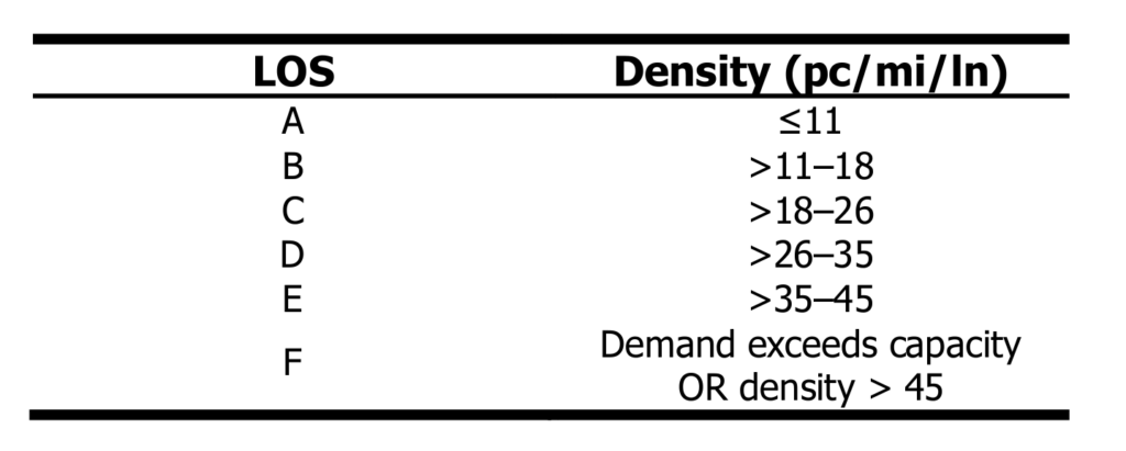
Freeway Merge and Diverge Segments

Similar to LOS scores for basic freeway and multi-lane highways, density is the primary consideration when scoring freeway merge and diverge segments.  LOS scores  are defined as:  

LOS A:  Operations are unrestricted, and merging or diverging is smooth with little disruption.  

LOS B : Minimal disruptions occur, merging and diverging is noticeable to through drivers.  

LOS C:  Traffic is somewhat disrupted, and drivers on both the ramps and freeway need to adjust their speed to allow for merging and diverging.  

LOS D:  All vehicles need to slow for merging or diverging to occur, and queues may begin forming on high volume ramps.  

LOS E:  Operating conditions are near or at capacity, and minor changes in demand or traffic may cause queueing on both the ramp and freeway.  

LOS F:   Demand exceeds capacity, and queues form on both the ramp and freeway. 

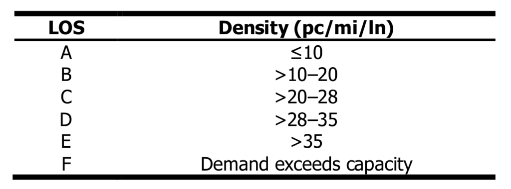
Two-Lane Highways

Two-lane highways differ greatly from multi-lane highways, because drivers are more limited in their mobility and speed. Any additional cars on the road can have significant impacts on traffic. For motorized vehicles, the three service measures used to determine LOS are: average travel speed (highway segment length divided by average travel time), percent time spent following (average time spent in groups behind slow vehicles), and percent of free-flow speed. On two-lane highways, there is also a bicycle LOS (BLOS) score, based on traveler perception. There are 5 considerations to the BLOS score: average effective width of the outside through lane, vehicle volumes, vehicle speeds, heavy vehicle volumes, and pavement conditions.  LOS scores  for motorized vehicles are defined as:  

LOS A:   High operating speeds at or near the FFS. Platooning is limited or unlikely, and motorists can pass easily. 

LOS B:   There is a balance between passing demand and capacity, and vehicle platooning occurs. There are small speed reductions. 

LOS C:  Speeds are noticeably reduced, and platoons occur for most vehicles. 

LOS D:  There is increased speed reduction, and significant platooning. Passing demand is high, but capacity is severely restricted, increasing percent time spent following. 

LOS E:  Speed is greatly reduced, and demand is almost at capacity, making passing impossible. At the lower end of LOS E, roads hit capacity. 

LOS F:  This occurs when the demand in at least one direction exceeds capacity, creating heavy congestion. 

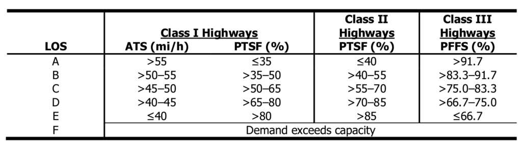
Urban Street Segments

Level of service scores for urban street segments are determined for motorized vehicles, pedestrians, bicycles, and transit, with the LOS score for motorized vehicles having different criteria and being more easily measured. The performance measures for motorized vehicles are travel speed for through vehicles and volume-to-capacity ratio for downstream through movement. LOS scores for pedestrian, bicycle, and transit modes are usually based on traveler perception, and can be calculated for specific links or segments.  LOS scores  for motorized vehicles are defined as:

LOS A:   Free flow operation with travel speeds exceeding 80% of the base free-flow speed. The volume-to-capacity ratio is not higher than 1.0, and there are no obstructions to maneuvering. 

LOS B:  Travel speed is between 67-80% of the base free-flow speed, and the volume-to-capacity ratio is not higher than 1.0. There are only slight restrictions for maneuvers. 

LOS C:   Travel speed is between 50-67% of the base free-flow speed, and the volume-to capacity ratio is not higher than 1.0. Longer queues at intersections may cause lower speeds. Maneuvers are more restricted than LOS B. 

LOS D:  Travel speed is between 40-50% of the base free-flow speed, and the volume-to-capacity ratio is not higher than 1.0. Any increase in flow will cause a significant decrease in travel speed and increased delay. 

LOS E:  Travel speed is between 30-40% of the base free-flow speed, and the volume-to-capacity ratio is no greater than 1.0. There is significant delay for motorists. 

LOS F:   Travel speed is 30% or less of the base free-flow speed, or the volume-to-capacity ratio is above 1.0. Traffic speed is extremely low, and there is high delay and queuing. 

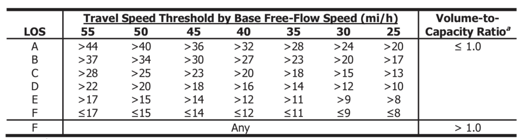
Signalized Intersections

Signalized intersections have an LOS score for motorized vehicles, pedestrians, bicycles, and transit, with the LOS score for motorized vehicles having different criteria and being more easily measured. LOS can be determined for whole intersections, each intersection approach, and each lane group. For lane groups, control delay and volume-to-capacity ratio are the primary performance measures considered. LOS scores for pedestrian, bicycle, and transit modes are usually based on traveler perception, and can include factors such as speed and crosswalk width.  LOS scores  for motorized vehicles are defined as: 

LOS A:   Control delay no higher than 10 s/veh and a volume-to-capacity ratio no higher than 1.0. Typically assigned when progression at the intersection is exceptional with high arrival on green, or there is a very short cycle length. 

LOS B:   Control delay between 10 and 20 s/veh and a volume-to-capacity ratio no higher than 1.0. Typically assigned when there is exceptional progression at the intersection or there is a short cycle length. More vehicles have to stop than LOS A. 

LOS C:   Control delay between 20 and 35 s/veh and a volume-to-capacity ratio no higher than 1.0. Typically assigned when progression at the intersection is good or the cycle length is average. Many vehicles have to stop, and individual cycle failures may start to occur. 

LOS D:   Control delay between 35 and 55 s/veh and a volume-to-capacity ratio no higher than 1.0. Typically assigned when progression is not effective or there is a long cycle length. Many vehicles have to stop, and individual cycle failures happen more regularly. 

LOS E:   Control delay between 55 and 80 s/veh and a volume-to-capacity ratio no higher than 1.0. Typically assigned when progression is not ideal and there is a long cycle length. Individual cycle failures happen frequently. 

LOS F:   Control delay is over 80 s/veh or the volume-to-capacity ratio is higher than 1.0. Typically assigned when progression is very bad and there is a long cycle length. Most cycles are not able to clear the queue. 

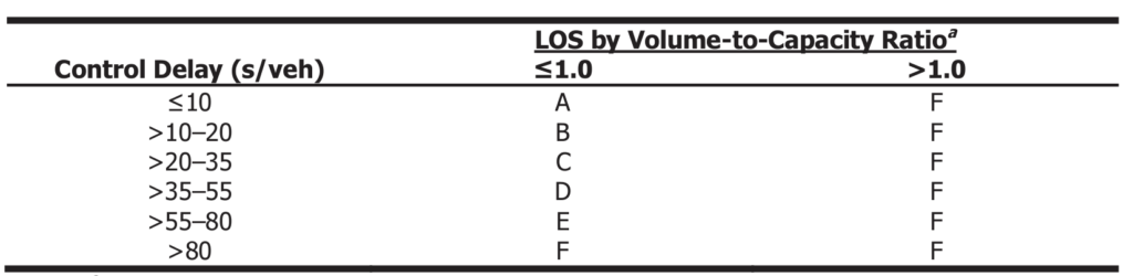
Off-Street Pedestrian and Bicycle Facilities

When determining LOS for on-street facilities, the pedestrian and bicyclist quality of service often reflects motorized traffic and how that traffic affects quality of service considerations, such as safety. When determining LOS for off-street facilities, three primary service measures include: pedestrian space (pedestrian only facilities), bicycle meeting and passing events per hour (pedestrian and bicycle facilities), and bicycle LOS (presence of bicyclists and road conditions for shared and exclusive bike paths). As cities move toward multimodal LOS scoring, pedestrian and bicycle considerations are becoming more important. 

LOS scores use a common set of definitions and grading scale to allow for easy assessment of a roadway’s quality of service, allowing agencies and planners to determine whether changes will improve or decrease traveler’s perceived quality of service. Different roadways have different LOS criteria, and newer, multimodal approaches are straying from car-centric scoring to include alternative modes of transport. 

Primary Source:  Highway Capacity Manual , Sixth Edition: A Guide for Multimodal Mobility Analysis 

Data collection methods, such as connected car trajectory data ,  available through  SMATS , can create data that has been color-coded by LOS, making data analyzation efficient and consistent.

Recent posts.

• SMATS Traffic Solutions Announces Partnership with TomTom 
• Speeding up the Supply Chain: A Guide for Real-Time Truck Data Collection and Sharing
• 5 Ways to Use Floating Car Data  
• 5 Reasons for Adding Floating Car Data to your Data Mix
• Connected Car Data: The Next Generation of Surrogate Safety Analytics

Privacy Overview

• Today's news
• Reviews and deals
• Climate change
• 2024 election
• Fall allergies
• Health news
• Mental health
• Sexual health
• Family health
• So mini ways
• Unapologetically
• Buying guides

Entertainment

• How to Watch
• My Portfolio
• Latest News
• Stock Market
• Biden Economy
• Stocks: Most Actives
• Stocks: Gainers
• Stocks: Losers
• Trending Tickers
• World Indices
• US Treasury Bonds Rates
• Top Mutual Funds
• Options: Highest Open Interest
• Options: Highest Implied Volatility
• Basic Materials
• Communication Services
• Consumer Cyclical
• Consumer Defensive
• Financial Services
• Industrials
• Real Estate
• Stock Comparison
• Advanced Chart
• Currency Converter
• Credit Cards
• Balance Transfer Cards
• Cash-back Cards
• Rewards Cards
• Travel Cards
• Credit Card Offers
• Best Free Checking
• Student Loans
• Personal Loans
• Car insurance
• Mortgage Refinancing
• Mortgage Calculator
• Morning Brief
• Market Domination
• Market Domination Overtime
• Asking for a Trend
• Opening Bid
• Stocks in Translation
• Lead This Way
• Good Buy or Goodbye?
• Financial Freestyle
• Capitol Gains
• Fantasy football
• Pro Pick 'Em
• College Pick 'Em
• Fantasy baseball
• Fantasy hockey
• Fantasy basketball
• Download the app
• Daily fantasy
• Scores and schedules
• GameChannel
• World Baseball Classic
• Premier League
• CONCACAF League
• Champions League
• Motorsports
• Horse racing
• Newsletters

New on Yahoo

• Privacy Dashboard

Yahoo Finance

American express global business travel reports strong q2 2024 financial results and raises 2024 free cash flow guidance.

NEW YORK, August 06, 2024 --( BUSINESS WIRE )--American Express Global Business Travel, which is operated by Global Business Travel Group, Inc. (NYSE: GBTG) ("Amex GBT" or the "Company"), a leading B2B software and services company for travel, expense, and meetings & events, today announced financial results for the second quarter ended June 30, 2024.

Second Quarter 2024 Highlights

Delivered Strong Financial Results

Revenue grew 6% year over year to $625 million.

Adjusted EBITDA grew 20% year over year to $127 million.

Strong Free Cash Flow generation of $49 million, representing growth of 148% year over year.

Controlled Costs & Drove Operating Leverage

2% Adjusted Operating Expense growth versus 6% revenue growth.

Operating leverage drove Adjusted EBITDA margin expansion of 240bps year over year.

Raised Free Cash Flow Guidance

Raised full-year 2024 Free Cash Flow Guidance to >$130 million (up from >$100 million).

Reiterated full-year 2024 revenue and Adjusted EBITDA guidance.

Lowered Interest Costs and Extended Debt Maturities

Lowered leverage ratio to 2.0x from 2.2x in the first quarter and 3.5x a year ago 1 .

July refinancing significantly lowers interest costs, extends maturities on all debt until 2031 and increases liquidity.

Continued Share Gains on a Strong Foundation

LTM Total New Wins Value of $3.3 billion, including $2.0 billion from SME.

97% LTM customer retention rate.

Paul Abbott, Amex GBT’s Chief Executive Officer, stated: "In the second quarter, we delivered strong Adjusted EBITDA growth, significant margin expansion and accelerated Free Cash Flow, and with our recent debt refinancing, we significantly lowered interest costs. We have a solid foundation with increasingly strong customer retention, and we continue to gain share while controlling costs. This puts us well on track to deliver against our full-year revenue and Adjusted EBITDA guidance and raise our full-year Free Cash Flow guidance."

Second Quarter 2024 Financial Summary

Second Quarter 2024 Financial Highlights (Changes compared to prior year period unless otherwise noted)

Revenue of $625 million increased $33 million, or 6%. Within this, Travel Revenue increased $27 million, or 6%, primarily due to 4% Transaction Growth and 5% TTV growth. Product and Professional Services Revenue increased $6 million, or 5%, primarily due to increased management fees and increased consulting and other professional services revenues. Revenue Yield of 8.1% was flat year over year.

Total operating expenses of $583 million decreased $7 million, or 1%. Continued investments in technology and content and increased cost of revenue to support Transaction Growth were offset by lower general & administrative and sales & marketing costs due to cost savings initiatives, including productivity improvements driven by artificial intelligence initiatives, in addition to decreased restructuring charges.

Adjusted Operating Expenses of $498 million increased $12 million, or 2%.

Net income was $27 million, an improvement of $82 million versus net loss of $55 million in the same period in 2023, primarily due to improvement in operating leverage from higher revenue, favorable fair value movements on earnout derivative liabilities, lower interest expense and benefit from income taxes.

Adjusted EBITDA of $127 million increased $21 million, or 20%. Revenue growth and operating leverage resulted in Adjusted EBITDA margin expansion of 240bps to 20%.

Net cash from operating activities totaled $73 million, an improvement of $27 million, or 57%, due to favorable net change in working capital, including benefit from the Egencia working capital optimization actions.

Free Cash Flow totaled $49 million, an improvement of $30 million, or 148%, due to the increase in net cash from operating activities and decreased use of cash for the purchase of property and equipment.

Net Debt: As of June 30, 2024, total debt, net of unamortized debt discount and debt issuance cost was $1,365 million, compared to $1,362 million as of December 31, 2023. Net Debt was $850 million as of June 30, 2024, compared to $886 million as of December 31, 2023. Leverage ratio was 2.0x as of June 30, 2024, down from 2.3x as of December 31, 2023. The cash balance was $515 million as of June 30, 2024, compared to $476 million as of December 31, 2023.

Raising Full-Year 2024 Free Cash Flow Guidance

Karen Williams, Amex GBT's Chief Financial Officer, stated: "In the second quarter, we continued to deliver strong Adjusted EBITDA growth with margin expansion and accelerated cash flow generation, all while investing to drive long-term, sustained growth. Our recent debt refinancing further strengthened our financial position, lowered interest costs, extending debt maturities to 2031 and increased liquidity with an upsized revolver. We remain confident that our focus on productivity and margin expansion will drive full-year Adjusted EBITDA growth between 18% and 32%, and expect Free Cash Flow generation in excess of $130 million in 2024."

The guidance below does not incorporate the impact of the previously announced CWT acquisition, which is expected to close in the first quarter of 2025.

Please refer to the section below titled "Reconciliation of Full-Year 2024 Adjusted EBITDA and Free Cash Flow Guidance" for a description of certain assumptions and risks associated with this guidance and reconciliation to GAAP.

Webcast Information

Amex GBT will host its second quarter 2024 investor conference call today at 9:00 a.m. E.T. The live webcast and accompanying slide presentation can be accessed on the Amex GBT Investor Relations website at investors.amexglobalbusinesstravel.com . A replay of the event will be available on the website for at least 90 days following the event.

Glossary of Terms

See the "Glossary of Terms" for the definitions of certain terms used within this press release.

Non-GAAP Financial Measures

The Company refers to certain financial measures that are not recognized under GAAP in this press release, including EBITDA, Adjusted EBITDA, Adjusted EBITDA Margin, Adjusted Operating Expenses, Free Cash Flow and Net Debt. See "Non-GAAP Financial Measures" below for an explanation of these non-GAAP financial measures and "Tabular Reconciliations for Non-GAAP Financial Measures" below for reconciliations of the non-GAAP financial measures to the comparable GAAP measures.

About American Express Global Business Travel

American Express Global Business Travel (Amex GBT) is the world’s leading B2B travel platform, providing software and services to manage travel, expenses, and meetings & events for companies of all sizes. We have built the most valuable marketplace in B2B travel to deliver unrivalled choice, value and experiences. With travel professionals and business partners in more than 140 countries, our solutions deliver savings, flexibility, and service from a brand you can trust – Amex GBT.

Visit amexglobalbusinesstravel.com for more information about Amex GBT. Follow @amexgbt on X (formerly known as Twitter), LinkedIn and Instagram.

B2B refers to business-to-business.

Customer retention rate is calculated based on Total Transaction Value (TTV).

CWT refers to CWT Holdings, LLC.

LTM refers to the last twelve months ended June 30, 2024.

Revenue Yield is calculated as total revenue divided by Total Transaction Value (TTV) for the same period.

SME refers to clients Amex GBT considers small-to-medium-sized enterprises, which Amex GBT generally defines as having an expected annual TTV of less than $30 million. This criterion can vary by country and customer needs and Amex GBT does not have products or services that are offered solely to one size customer or another.

Total New Wins Value is calculated using expected annual average Total Transaction Value (TTV) over the contract term from all new client wins over the last twelve months.

Total Transaction Value or TTV refers to the sum of the total price paid by travelers for air, hotel, rail, car rental and cruise bookings, including taxes and other charges applied by suppliers at point of sale, less cancellations and refunds.

Transaction Growth represents year-over-year increase or decrease as a percentage of the total transactions, including air, hotel, car rental, rail or other travel-related transactions, recorded at the time of booking, and is calculated on a net basis to exclude cancellations, refunds and exchanges. To calculate year-over-year growth or decline, we compare the total number of transactions in the comparative previous period/ year to the total number of transactions in the current period/year in percentage terms. For the six months ended June 30, 2024, we have presented Transaction Growth on a net basis to exclude cancellations, refunds and exchanges as management believes this better aligns Transaction Growth with the way we measure TTV and earn revenue. Prior period Transaction Growth percentages have been recalculated and represented to conform to current period presentation.

We report our financial results in accordance with GAAP. Our non-GAAP financial measures are provided in addition, and should not be considered as an alternative, to other performance or liquidity measures derived in accordance with GAAP. Non-GAAP financial measures have limitations as analytical tools, and you should not consider them either in isolation or as a substitute for analyzing our results as reported under GAAP. In addition, because not all companies use identical calculations, the presentations of our non-GAAP financial measures may not be comparable to other similarly titled measures of other companies and can differ significantly from company to company.

Management believes that these non-GAAP financial measures provide users of our financial information with useful supplemental information that enables a better comparison of our performance or liquidity across periods. In addition, we use certain of these non-GAAP financial measures as performance measures as they are important metrics used by management to evaluate and understand the underlying operations and business trends, forecast future results and determine future capital investment allocations. We also use certain of our non-GAAP financial measures as indicators of our ability to generate cash to meet our liquidity needs and to assist our management in evaluating our financial flexibility, capital structure and leverage. These non-GAAP financial measures supplement comparable GAAP measures in the evaluation of the effectiveness of our business strategies, to make budgeting decisions, and/or to compare our performance and liquidity against that of other peer companies using similar measures.

We define EBITDA as net income (loss) before interest income, interest expense, gain (loss) on early extinguishment of debt, benefit from (provision for) income taxes and depreciation and amortization.

We define Adjusted EBITDA as net income (loss) before interest income, interest expense, gain (loss) on early extinguishment of debt, benefit from (provision for) income taxes and depreciation and amortization and as further adjusted to exclude costs that management believes are non-core to the underlying business of the Company, consisting of restructuring, exit and related charges, integration costs, costs related to mergers and acquisitions, non-cash equity-based compensation and related employer taxes, long-term incentive plan costs, certain corporate costs, fair value movements on earnout derivative liabilities, foreign currency gains (losses), non-service components of net periodic pension benefit (costs) and gains (losses) on disposal of businesses.

We define Adjusted EBITDA Margin as Adjusted EBITDA divided by revenue.

We define Adjusted Operating Expenses as total operating expenses excluding depreciation and amortization and costs that management believes are non-core to the underlying business of the Company, consisting of restructuring, exit and related charges, integration costs, costs related to mergers and acquisitions, non-cash equity-based compensation and related employer taxes, long-term incentive plan costs and certain corporate costs.

EBITDA, Adjusted EBITDA, Adjusted EBITDA Margin and Adjusted Operating Expenses are supplemental non-GAAP financial measures of operating performance that do not represent and should not be considered as alternatives to net income (loss) or total operating expenses, as determined under GAAP. In addition, these measures may not be comparable to similarly titled measures used by other companies.

These non-GAAP measures have limitations as analytical tools, and these measures should not be considered in isolation or as a substitute for analysis of the Company’s results or expenses as reported under GAAP. Some of these limitations are that these measures do not reflect:

changes in, or cash requirements for, our working capital needs or contractual commitments;

our interest expense, or the cash requirements to service interest or principal payments on our indebtedness;

our tax expense, or the cash requirements to pay our taxes;

recurring, non-cash expenses of depreciation and amortization of property and equipment and definite-lived intangible assets and, although these are non-cash expenses, the assets being depreciated and amortized may have to be replaced in the future;

the non-cash expense of stock-based compensation, which has been, and will continue to be for the foreseeable future, an important part of how we attract and retain our employees and a significant recurring expense in our business;

restructuring, mergers and acquisition and integration costs, all of which are intrinsic of our acquisitive business model; and

impact on earnings or changes resulting from matters that are non-core to our underlying business, as we believe they are not indicative of our underlying operations.

EBITDA, Adjusted EBITDA, Adjusted EBITDA Margin and Adjusted Operating Expenses should not be considered as a measure of liquidity or as a measure determining discretionary cash available to us to reinvest in the growth of our business or as measures of cash that will be available to us to meet our obligations.

We believe that the adjustments applied in presenting EBITDA, Adjusted EBITDA, Adjusted EBITDA Margin and Adjusted Operating Expenses are appropriate to provide additional information to investors about certain material non-cash and other items that management believes are non-core to our underlying business.

We use these measures as performance measures as they are important metrics used by management to evaluate and understand the underlying operations and business trends, forecast future results and determine future capital investment allocations. These non-GAAP measures supplement comparable GAAP measures in the evaluation of the effectiveness of our business strategies, to make budgeting decisions, and to compare our performance against that of other peer companies using similar measures. We also believe that EBITDA, Adjusted EBITDA, Adjusted EBITDA Margin and Adjusted Operating Expenses are helpful supplemental measures to assist potential investors and analysts in evaluating our operating results across reporting periods on a consistent basis.

We define Free Cash Flow as net cash from (used in) operating activities, less cash used for additions to property and equipment.

We believe Free Cash Flow is an important measure of our liquidity. This measure is a useful indicator of our ability to generate cash to meet our liquidity demands. We use this measure to conduct and evaluate our operating liquidity. We believe it typically presents an alternate measure of cash flow since purchases of property and equipment are a necessary component of our ongoing operations and it provides useful information regarding how cash provided by operating activities compares to the property and equipment investments required to maintain and grow our platform. We believe Free Cash Flow provides investors with an understanding of how assets are performing and measures management’s effectiveness in managing cash.

Free Cash Flow is a non-GAAP measure and may not be comparable to similarly named measures used by other companies. This measure has limitations in that it does not represent the total increase or decrease in the cash balance for the period, nor does it represent cash flow for discretionary expenditures. This measure should not be considered as a measure of liquidity or cash flow from operations as determined under GAAP. This measure is not a measurement of our financial performance under GAAP and should not be considered in isolation or as an alternative to net income (loss) or any other performance measures derived in accordance with GAAP or as an alternative to cash flow from operating activities as a measure of liquidity.

We define Net Debt as total debt outstanding consisting of the current and non-current portion of long-term debt, net of unamortized debt discount and unamortized debt issuance costs, minus cash and cash equivalents. Net Debt is a non-GAAP measure and may not be comparable to similarly named measures used by other companies. This measure is not a measurement of our indebtedness as determined under GAAP and should not be considered in isolation or as an alternative to assess our total debt or any other measures derived in accordance with GAAP or as an alternative to total debt. Management uses Net Debt to review our overall liquidity, financial flexibility, capital structure and leverage. Further, we believe that certain debt rating agencies, creditors and credit analysts monitor our Net Debt as part of their assessment of our business.

Tabular Reconciliations for Non-GAAP Measures

Reconciliation of net income (loss) to EBITDA and Adjusted EBITDA:

Reconciliation of total operating expenses to Adjusted Operating Expenses:

Reconciliation of net cash from operating activities to Free Cash Flow:

Reconciliation of Net Debt:

Reconciliation of Full-Year 2024 Adjusted EBITDA and Free Cash Flow Guidance

The Company’s full-year 2024 guidance considers various material assumptions. Because the guidance is forward-looking and reflects numerous estimates and assumptions with respect to future industry performance under various scenarios as well as assumptions for competition, general business, economic, market and financial conditions and matters specific to the business of Amex GBT, all of which are difficult to predict and many of which are beyond the control of Amex GBT, actual results may differ materially from the guidance due to a number of factors, including the ultimate inaccuracy of any of the assumptions described above and the risks and other factors discussed in the section entitled "Forward-Looking Statements" below and the risk factors in the Company’s SEC filings.

The guidance below does not incorporate the impact of the CWT acquisition, which is expected to close in the first quarter of 2025.

Adjusted EBITDA guidance for the year ending December 31, 2024 consists of expected net loss for the year ending December 31, 2024, adjusted for: (i) interest expense of approximately $120 million; (ii) loss on extinguishment of debt of approximately $40 million; (iii) income taxes of approximately $60-70 million; (iv) depreciation and amortization of property and equipment of approximately $180-185 million; (v) restructuring costs of approximately $25-30 million; (vi) integration expenses and costs related to mergers and acquisitions of approximately $60-65 million; (vii) non-cash equity-based compensation of approximately $80-85 million, and; (viii) other adjustments, including long-term incentive plan costs, legal and professional services costs, non-service component of our net periodic pension benefit (cost) related to our defined benefit pension plans and foreign exchange gains and losses of approximately $10-20 million. We are unable to reconcile Adjusted EBITDA to net income (loss) determined under U.S. GAAP due to the unavailability of information required to reasonably predict certain reconciling items such as impairment of long-lived assets and right-of-use assets and fair value movement on earnout derivative liabilities and the related tax impact of these adjustments. The exact amount of these adjustments is not currently determinable but may be significant.

Free Cash Flow guidance for the year ending December 31, 2024 consists of expected net cash from operating activities of greater than $250-280 million less purchase of property and equipment of approximately $120-130 million.

Forward-Looking Statements

This release contains statements that are forward-looking and as such are not historical facts. This includes, without limitation, statements regarding our financial position, business strategy, the plans and objectives of management for future operations and full-year guidance. These statements constitute projections, forecasts and forward-looking statements within the meaning of the Private Securities Litigation Reform Act of 1995. The words "anticipate," "believe," "continue," "could," "estimate," "expect," "intend," "may," "might," "plan," "possible," "potential," "predict," "project," "should," "will," "would" and similar expressions may identify forward-looking statements, but the absence of these words does not mean that a statement is not forward-looking.

The forward-looking statements contained in this release are based on our current expectations and beliefs concerning future developments and their potential effects on us. There can be no assurance that future developments affecting us will be those that we have anticipated. These forward-looking statements involve a number of risks, uncertainties (some of which are beyond our control) or other assumptions that may cause actual results or performance to be materially different from those expressed or implied by these forward-looking statements. These risks and uncertainties include, but are not limited to, the following risks, uncertainties and other factors: (1) changes to projected financial information or our ability to achieve our anticipated growth rate and execute on industry opportunities; (2) our ability to maintain our existing relationships with customers and suppliers and to compete with existing and new competitors; (3) various conflicts of interest that could arise among us, affiliates and investors; (4) our success in retaining or recruiting, or changes required in, our officers, key employees or directors; (5) factors relating to our business, operations and financial performance, including market conditions and global and economic factors beyond our control; (6) the impact of geopolitical conflicts, including the war in Ukraine and the conflicts in the Middle East, as well as related changes in base interest rates, inflation and significant market volatility on our business, the travel industry, travel trends and the global economy generally; (7) the sufficiency of our cash, cash equivalents and investments to meet our liquidity needs; (8) the effect of a prolonged or substantial decrease in global travel on the global travel industry; (9) political, social and macroeconomic conditions (including the widespread adoption of teleconference and virtual meeting technologies which could reduce the number of in-person business meetings and demand for travel and our services); (10) the effect of legal, tax and regulatory changes; (11) our ability to complete any potential acquisition in a timely manner or at all; (12) our ability to recognize the anticipated benefits of any future acquisition, which may be affected by, among other things, competition, the ability of the combined company to grow and manage growth profitably, maintain relationships with customers and suppliers and retain key employees; (13) risks related to, or unexpected liabilities that arise in connection with, any future acquisition or the integration of any acquisition; and (14) other risks and uncertainties described in the Company’s Form 10-K, filed with the SEC on March 13, 2024, and in the Company’s other SEC filings. Should one or more of these risks or uncertainties materialize, or should any of our assumptions prove incorrect, actual results may vary in material respects from those projected in these forward-looking statements. We undertake no obligation to update or revise any forward-looking statements, whether as a result of new information, future events or otherwise, except as may be required under applicable securities laws.

An investment in Global Business Travel Group, Inc. is not an investment in American Express. American Express shall not be responsible in any manner whatsoever for, and in respect of, the statements herein, all of which are made solely by Global Business Travel Group, Inc.

_________________ 1 Leverage ratio is calculated as Net Debt / LTM Adjusted EBITDA and is different than leverage ratio defined in our amended and restated senior secured credit agreement.

View source version on businesswire.com: https://www.businesswire.com/news/home/20240806574977/en/

Media: Martin Ferguson Vice President Global Communications and Public Affairs [email protected]

Investors: Jennifer Thorington Vice President Investor Relations [email protected]

Advertisement

Supported by

Britain’s Violent Riots: What We Know

Officials had braced for more unrest on Wednesday, but the night’s anti-immigration protests were smaller, with counterprotesters dominating the streets instead.

• Share full article

By Lynsey Chutel

After days of violent rioting set off by disinformation around a deadly stabbing rampage, the authorities in Britain had been bracing for more unrest on Wednesday. But by nightfall, large-scale anti-immigration demonstrations had not materialized, and only a few arrests had been made nationwide.

Instead, streets in cities across the country were filled with thousands of antiracism protesters, including in Liverpool, where by late evening, the counterdemonstration had taken on an almost celebratory tone.

Over the weekend, the anti-immigration protests, organized by far-right groups, had devolved into violence in more than a dozen towns and cities. And with messages on social media calling for wider protests and counterprotests on Wednesday, the British authorities were on high alert.

With tensions running high, Prime Minister Keir Starmer’s cabinet held emergency meetings to discuss what has become the first crisis of his recently elected government. Some 6,000 specialist public-order police officers were mobilized nationwide to respond to any disorder, and the authorities in several cities and towns stepped up patrols.

Wednesday was not trouble-free, however.

In Bristol, the police said there was one arrest after a brick was thrown at a police vehicle and a bottle was thrown. In the southern city of Portsmouth, police officers dispersed a small group of anti-immigration protesters who had blocked a roadway. And in Belfast, Northern Ireland, where there have been at least four nights of unrest, disorder continued, and the police service said it would bring in additional officers.

But overall, many expressed relief that the fears of wide-scale violence had not been realized.

Here’s what we know about the turmoil in Britain.

Where has the unrest taken place?

Protesters over the weekend took to the streets of a dozen cities across Britain, most of them in England. Trouble broke out from Aldershot in the south to Sunderland in the north and Liverpool in the west. Belfast, in Northern Ireland, was also drawn into the fray.

In some cases, the protesters were merely unruly, but in others the violence was more pronounced.

Where arrests have been reported

On Sunday, rioters set upon a hotel that was housing asylum seekers in the town of Rotherham, in northern England, breaking windows before surging inside as the police struggled to control them. No guests were injured in the melee, the police said.

In Middlesbrough, a group of rioters, some masked, hurled bottles and rocks at officers. Cars were set on fire, and at least nine people were arrested. On Saturday, a library and a food bank were set ablaze in Liverpool as groups damaged and looted businesses, and in Hull, fires were set and storefronts smashed in the city center.

Dozens of police officers were injured, including some who required trips to the hospital.

What set off the protests?

The unrest began after a teenager wielding a knife attacked a children’s dance class early last week in the seaside town of Southport, which is near Liverpool. Three children were killed, and eight were wounded.

The suspect was born and raised in Britain, but online rumors soon circulated that he was an undocumented immigrant. To counter those false claims, the authorities took the unusual step of publicly identifying him. The BBC has reported that the suspect’s parents are from Rwanda. The police have not disclosed a motive for the stabbing attack.

But with migration a flashpoint issue in Britain, especially on the far right, the rumors were all it took to set off violence.

Extremist groups urged their followers to take to the streets, and on the day after the stabbings, they began to do so, starting in Southport.

How have the authorities responded?

The weekend riots prompted a heavy police response. Nearly 4,000 additional officers were deployed, a law enforcement association said. And a government order gave officers in some places special powers to disperse any gatherings or “antisocial behavior,” the police said in a statement .

More than 400 people have been arrested, and about 100 have been charged, Mr. Starmer said after an emergency cabinet meeting on Tuesday — the second in two days.

The prime minister, who has characterized the riots as “far-right thuggery,” encouraged prosecutors to name and shame those convicted to dissuade others from joining the violent rampages.

“I’m now expecting substantive sentencing before the end of the week,” Mr. Starmer said. “That should send a very powerful message to anybody involved, either directly or online, that you are likely to be dealt with within a week and that nobody, but nobody, should involve themselves in this disorder.”

BJ Harrington, the head of public order for Britain’s National Police Chiefs’ Council, said that online disinformation had been “a huge driver of this appalling violence.”

Intelligence teams, detectives and neighborhood officers, Mr. Harrington said, were working to identify the people fomenting the violence.

“They won’t win,” he said.

How are the authorities handling online incitement?

Social media has acted as an accelerant throughout the protests, with disinformation fueling far-right and anti-immigrant groups . Britain and other democracies have found that policing the internet is legally murky terrain, with individual rights and free speech protections balanced against a desire to block harmful material .

In his remarks on Tuesday, Mr. Starmer said that some arrests involved people accused of inciting violence online.

The first person to be convicted over online posts since the riots, according to the Crown Prosecution Service , was a 28-year-old man from Leeds who posted messages on Facebook about attacking a hotel that housed asylum seekers. It said that the man, Jordan Parlour, had pleaded guilty and been convicted of using threatening words or behavior to stir up racial hatred.

Mr. Starmer has called out social media companies over misinformation on their platforms, but holding them accountable could be tricky. Britain adopted a law last year that requires social media companies to introduce protections for child safety and to prevent and quickly remove illegal content like terrorism propaganda and revenge pornography. The law is less clear about how companies must treat misinformation and incendiary language.

What are the political implications?

The riots are the first political crisis for Mr. Starmer, who took office a month ago after his Labour Party defeated the Conservatives, who had been in government for 14 years.

While in power, the Conservatives tried to capitalize on public unhappiness over immigration, vowing to reduce it (though failing to do so). But in recent days they joined Labour in condemning the violent protests.

Former Prime Minister Rishi Sunak, now the opposition leader, said the unrest had “nothing to do with the tragedy in Southport.” The police, he said, have “our full support to deal with these criminals swiftly.”

Megan Specia contributed reporting.

Lynsey Chutel covers South Africa and the countries that make up southern Africa from Johannesburg. More about Lynsey Chutel